Problem Set 06

Background

We will again use the hate crimes data we used in Problem Set 05. The FiveThirtyEight article about those data are in the Jan 23, 2017 “Higher Rates Of Hate Crimes Are Tied To Income Inequality.” This week, we will use these data to run regression models with a single categorical predictor (explanatory) variable and a single numeric predictor (explanatory) variable.

Setup

First load the necessary packages:

R Code

library(ggplot2)
library(dplyr)
library(moderndive)
library(readr)

The following code uses the function read_csv() to read in the data and store the information in an object named hate_crimes.

R Code

url <- "http://bit.ly/2ItxYg3"
if(!dir.exists("./data/")){
  dir.create("./data/")
  }
if(!file.exists("./data/hate_crimes.csv")){
    download.file(url, destfile = "./data/hate_crimes.csv")
  }
hate_crimes <- read_csv("./data/hate_crimes.csv")

Next, let’s explore the hate_crimes data set using the glimpse() function from the dplyr package:

glimpse(hate_crimes)

Rows: 51
Columns: 9
$ state            <chr> "New Mexico", "Maine", "New York", "Illinois", "Delaw…
$ median_house_inc <chr> "low", "low", "low", "low", "high", "high", "high", "…
$ share_pop_metro  <dbl> 0.69, 0.54, 0.94, 0.90, 0.90, 1.00, 0.87, 0.86, 0.97,…
$ hs               <dbl> 83, 90, 85, 86, 87, 85, 89, 90, 81, 91, 89, 89, 87, 8…
$ hate_crimes      <dbl> 0.295, 0.616, 0.351, 0.195, 0.323, 0.095, 0.833, 0.67…
$ trump_support    <chr> "low", "low", "low", "low", "low", "low", "low", "low…
$ unemployment     <chr> "high", "low", "low", "high", "low", "high", "high", …
$ urbanization     <chr> "low", "low", "high", "high", "high", "high", "high",…
$ income           <dbl> 46686, 51710, 54310, 54916, 57522, 58633, 58875, 5906…

You should also examine the data in the data viewer.

Each case/row in these data is a state in the US. This week we will consider the response variable income, which is the numeric variable of median income of households in each state.

We will use

• A categorical explanatory variable urbanization: level of urbanization in a region
• A numerical explanatory variable share_pop_hs: the percentage of adults 25 and older with a high school degree

Income, Education and Urbanization

We will start by modeling the relationship between:

• \(y\): Median household income in 2016
• \(x_1\): numerical variable percent of adults 25 and older with a high-school degree, contained in the hs variable
  
• \(x_2\): categorical variable level of urbanization in a state: low, or high, as contained in the variable urbanization

Exploratory Data Analysis

We will start by creating a scatterplot showing:

• Median household income on the \(y\) axis
• Percent of adults 25 or older with a high school degree on the \(x\) axis
• The points colored by the variable urbanization
• A line of best fit (regression line) for each level of the variable urbanization (one for “low”, one for “high”)

R Code

ggplot(data = hate_crimes, 
       aes(y = income, x = hs, color = urbanization)) +
  geom_point()+ 
  geom_smooth(method = "lm", se = FALSE) + 
  labs(
    x = "Percent of adults with high-school degree", 
    y = "Median household income in USD $", 
    title = "Income versus education in states with 
    differing levels of urbanization") + 
  theme_bw() + 
  theme(plot.title = element_text(hjust = 0.5))

Figure 1: Median household income versus percent of adults with high-school degree in states with differing levels of urbanization

Problem 1

Do you think the relationship between hs and income is strong or weak, linear or non-linear in Figure 1?

Problem 1 Answers

• Delete this and put your text answer here.

Problem 2

Which regression line (high urbanization or low urbanization) in Figure 1 has the larger intercept? Answer the question using the actual intercepts from the statistical model. Store the results of the lm() function in mod_full using the appropriate predictors to obtain the regression models depicted in Figure 1. Use either kable() from the knitr package or get_regression_table() from the moderndive package on mod_full. Make sure to format the intercepts in your answer using appropriate units.

Problem 2 Answers

# Type your code and comments inside the code chunk

• Delete this and put your text answer here.

Problem 3

Does the slope look fairly similar (parallel) for the two levels of urbanization?

Problem 3 Answers

• Delete this and put your text answer here.

Problem 4

Based on the data visualization in Figure 1, and your answer to 3, do you think it would be best to run a “parallel slopes” model (i.e. a model that estimates one shared slope for the two levels of urbanization), or a more complex “interaction model” (i.e. a model that estimates a separate slope for the two levels of urbanization)?

Problem 4 Answers

• Delete this and put your text answer here.

# Type your code and comments inside the code chunk

Problem 5

Create a data visualization comparing median household income at “low” and “high” levels of urbanization (you do not need to include the hs variable in this plot). Please include axis labels and and title.

Problem 5 Answers

# Type your code and comments inside the code chunk

Problem 6

Run a linear regression model that examines the relationship between household income (as response variable), and high-school education (hs), and urbanization as explanatory variables. Store the results of your model in an object named med_income_model. Generate the regression table using the get_regression_table() function from the moderndive package. Create a graph of the equations stored in med_income_model. Use appropriate labels for the \(x-\) and \(y-\) axes as well as a title in your graph.

Problem 6 Answers

library(scales)  # Used to format numbers and for dollars
# Type your code and comments inside the code chunk

# Type your code and comments here

Problem 7

Is the intercept the same for the states with a “low” and “high” level of urbanization? Is the slope the same? (look at the data visualization created in Problem 6 to help with this!)

Problem 7 Answers

• Delete this and put your text answer here.

Problem 8

What is the slope for the regression line of the states with a “high” level of urbanization? What is the intercept? Be sure to format your answers with appropriate units.

Problem 8 Answers

# Type your code and comments inside the code chunk

• Delete this and put your text answer here.

• Delete this and put your text answer here.

Problem 9

What is the slope for the regression line of the states with a “low” level of urbanization? What is the intercept? Be sure to format your answers with appropriate units.

Problem 9 Answers

• Delete this and put your text answer here.

• Delete this and put your text answer here.

Problem 10

Based on your regression table output (and the data visualizations), is median household income greater in states that have lower or higher levels of urbanization? By how much? Be sure to format your answer with appropriate units.

Problem 10 Answers

• Delete this and put your text answer here.

Problem 11

For every increase in 1 percentage point of high-school educated adults, what is the associated increase in the median household income of a state? Be sure to format your answer with appropriate units.

Problem 11 Answers

• Delete this and put your text answer here.

Problem 12

The regression equation for med_income_model is given below. Write the regression equation for a US state in which urbanization is “high”.

\[\widehat{\text{income}} = -113,725 + 1986.79 \times \text{hs} -7333.33 \times 1_{\text{low urbanization}}(\text{x})\]

Problem 12 Answers

• Your \(LaTeX\) answer here.

Problem 13

What would you predict as the median household income for a state with a high level of urbanization, in which 85% of the share of adults have a high school degree? Be sure to format your answer with appropriate units.

Problem 13 Answers

# Type your code and comments inside the code chunk

• Delete this and put your text answer here.

Problem 14

What would you predict as the median household income for a state with a low level of urbanization, in which 85% of the share of adults have a high school degree? Be sure to format your answer with appropriate units.

Problem 14 Answers

# Type your code and comments inside the code chunk

• Delete this and put your text answer here.

Problem 15

What would you predict as the median household income for a state with a low level of urbanization, in which 30% of adults have a high school degree?

Problem 15 Answers

• Delete this and put your text answer here.

Problem 16

What was the observed income value for Maine (row 2)? What was the prediction for Maine according to our model (med_income_model)? What is the residual? Did our model over or underestimate the median income for this state? Be sure to format your answers with appropriate units.

Problem 16 Answers

# Type your code and comments inside the code chunk

• Delete this and put your text answer here.

• Delete this and put your text answer here.

• Delete this and put your text answer here.

• Delete this and put your text answer here.

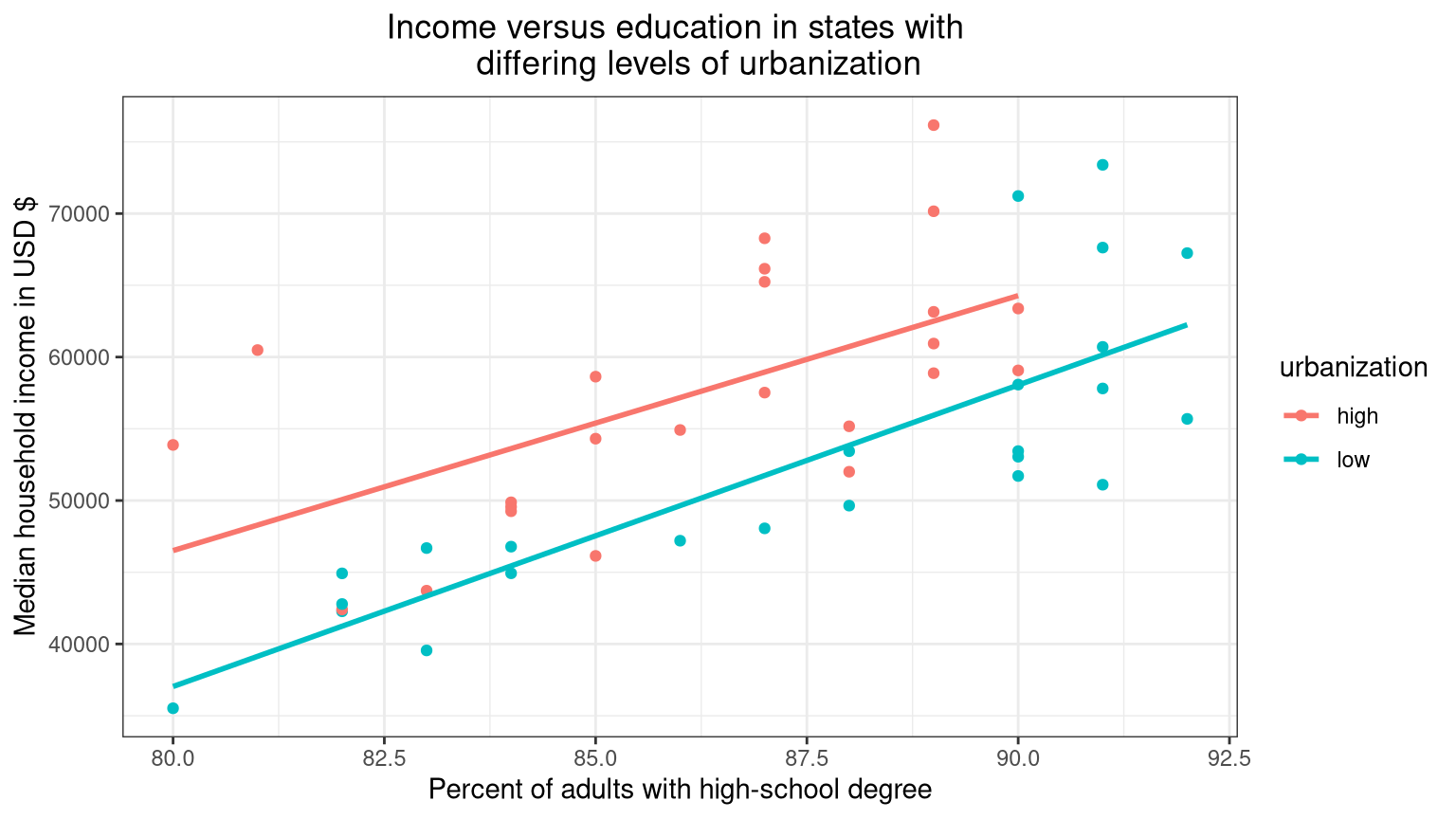
Independent Analysis

Figure 2: Vole in the wild

You will now use the tools you have learned, and a new data set to solve a conservation problem.

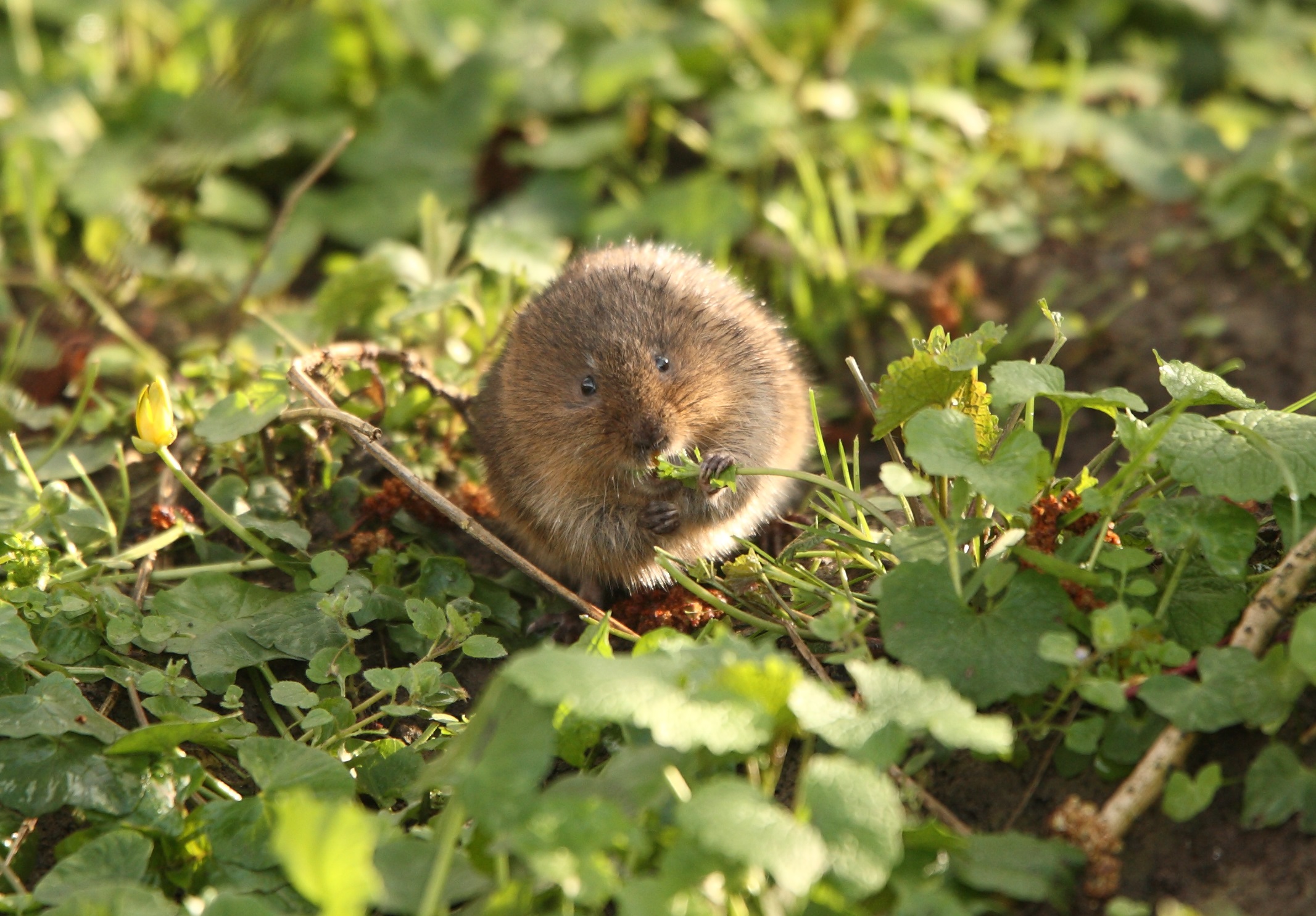
Wildlife biologists are interested in managing/protecting habitats for a declining species of vole, but are not sure about what habitats it prefers. Two things that biologists can easily control with management is percent cover of vegetation, and where habitat improvements occur (i.e. is it important to create/protect habitat in moist or dry sites, etc). To help inform habitat management of this vole species, the researchers in this study counted the number of voles at 56 random study sites. At each site, they measured percent cover of vegetation, and recorded whether a site had moist or dry soil.

The data are read into the object vole_trapping using the read_csv() function below.

R Code

url <- "http://bit.ly/2IgDF0E"
if(!dir.exists("./data/")){
  dir.create("./data/")
  }
if(!file.exists("./data/vole_trapping.csv")){
    download.file(url, destfile = "./data/vole_trapping.csv")
  }
vole_trapping <- read_csv("./data/vole_trapping.csv")

The data contains the variables:

• site for the id of each random study site (each case or row is a survey/trapping site)
• voles for the vole count at each site
• veg for the percent cover of vegetation at each site
• soil identifying a site as “moist” or “dry”

Problem 17

Generate a regression model with voles as the response variable y and veg and soil as explanatory variables. Store the model in an object named voles_mod. Use the results of the model to answer the following questions based on the available data. Create a data visualization (parallel slopes) to help answer the questions.

Problem 17 Answers

# Type your code and comments inside the code chunk

Problem 18

Would you recommend to a manager that they try to protect sites with high or low vegetation cover? Why?

Problem 18 Answers

• Delete this and put your text answer here.

Problem 19

Dry sites are typically a lot less money to purchase and maintain for conservation organizations. Thus, if a conservation organization decides to purchase a few dry sites, roughly what percent cover of vegetation do they need to maintain on these sites (at a minimum) to support a population of about 30 voles at the site?

Problem 19 Answers

• Delete this and put your text answer here.

# Type your code and comments inside the code chunk

Problem 20

The Nature Conservancy is looking at purchasing a site for this species (in the same study area) that has moist soil and 40% vegetation cover. Using the regression equation what would you predict as the possible vole population the site might be able to support?

Problem 20 Answers

# Type your code and comments inside the code chunk

• Delete this and put your text answer here.

Turning in Your Work

You will need to make sure you commit and push all of your changes to the github education repository where you obtained the lab.

Tip

• Make sure you render a final copy with all your changes and work.
• Look at your final html file to make sure it contains the work you expect and is formatted properly.

Logging out of the Server

There are many statistics classes and students using the Server. To keep the server running as fast as possible, it is best to sign out when you are done. To do so, follow all the same steps for closing Quarto document:

Tip

• Save all your work.
• Click on the orange button in the far right corner of the screen to quit R
• Choose don’t save for the Workspace image
• When the browser refreshes, you can click on the sign out next to your name in the top right.
• You are signed out.

sessionInfo()

R version 4.4.2 (2024-10-31)
Platform: x86_64-redhat-linux-gnu
Running under: Red Hat Enterprise Linux 9.5 (Plow)

Matrix products: default
BLAS/LAPACK: FlexiBLAS OPENBLAS-OPENMP;  LAPACK version 3.9.0

locale:
 [1] LC_CTYPE=en_US.UTF-8       LC_NUMERIC=C              
 [3] LC_TIME=en_US.UTF-8        LC_COLLATE=en_US.UTF-8    
 [5] LC_MONETARY=en_US.UTF-8    LC_MESSAGES=en_US.UTF-8   
 [7] LC_PAPER=en_US.UTF-8       LC_NAME=C                 
 [9] LC_ADDRESS=C               LC_TELEPHONE=C            
[11] LC_MEASUREMENT=en_US.UTF-8 LC_IDENTIFICATION=C       

time zone: America/New_York
tzcode source: system (glibc)

attached base packages:
[1] stats     graphics  grDevices utils     datasets  methods   base     

other attached packages:
[1] readr_2.1.5      moderndive_0.7.0 dplyr_1.1.4      ggplot2_3.5.1   
[5] scales_1.3.0     knitr_1.49      

loaded via a namespace (and not attached):
 [1] generics_0.1.3       tidyr_1.3.1          lattice_0.22-6      
 [4] stringi_1.8.4        hms_1.1.3            digest_0.6.37       
 [7] magrittr_2.0.3       evaluate_1.0.3       grid_4.4.2          
[10] timechange_0.3.0     fastmap_1.2.0        Matrix_1.7-1        
[13] operator.tools_1.6.3 jsonlite_1.8.9       backports_1.5.0     
[16] mgcv_1.9-1           purrr_1.0.2          infer_1.0.7         
[19] cli_3.6.3            rlang_1.1.4          crayon_1.5.3        
[22] splines_4.4.2        bit64_4.5.2          munsell_0.5.1       
[25] withr_3.0.2          yaml_2.3.10          tools_4.4.2         
[28] parallel_4.4.2       tzdb_0.4.0           colorspace_2.1-1    
[31] broom_1.0.7          vctrs_0.6.5          R6_2.5.1            
[34] lifecycle_1.0.4      lubridate_1.9.4      snakecase_0.11.1    
[37] stringr_1.5.1        htmlwidgets_1.6.4    bit_4.5.0.1         
[40] vroom_1.6.5          janitor_2.2.1        pkgconfig_2.0.3     
[43] pillar_1.10.1        gtable_0.3.6         glue_1.8.0          
[46] xfun_0.50            tibble_3.2.1         tidyselect_1.2.1    
[49] rstudioapi_0.17.1    farver_2.1.2         nlme_3.1-166        
[52] htmltools_0.5.8.1    labeling_0.4.3       rmarkdown_2.29      
[55] formula.tools_1.7.1  compiler_4.4.2