Correlation
The correlation coefficient , denoted by \(r\) , measures the direction and strength of the linear relationship between two numerical variables. Is is given by the equation
\[
r = \frac{1}{(n-1)}\sum_{i=1}^n\left(\frac{x_i - \bar{x}}{s_x}\right)\left(\frac{y_i - \bar{y}}{s_y}\right)
\tag{1}\]
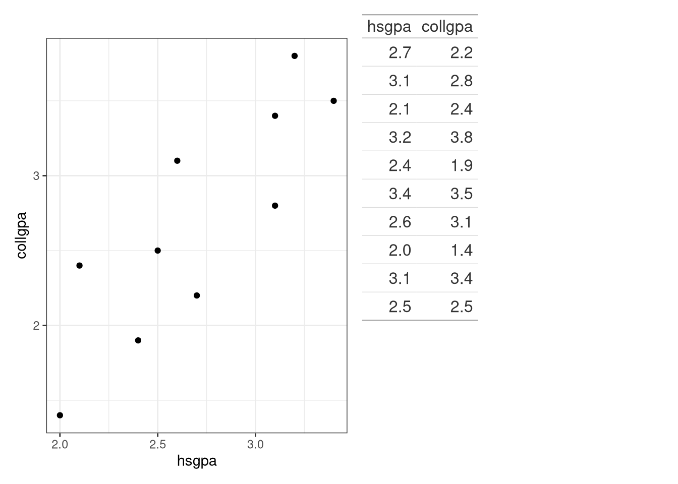
Following are the high school GPAs and the college GPAs at the end of the freshman year for ten different students from the Gpa data set of the BSDA package.
2.7
2.2
3.1
2.8
2.1
2.4
3.2
3.8
2.4
1.9
3.4
3.5
2.6
3.1
2.0
1.4
3.1
3.4
2.5
2.5
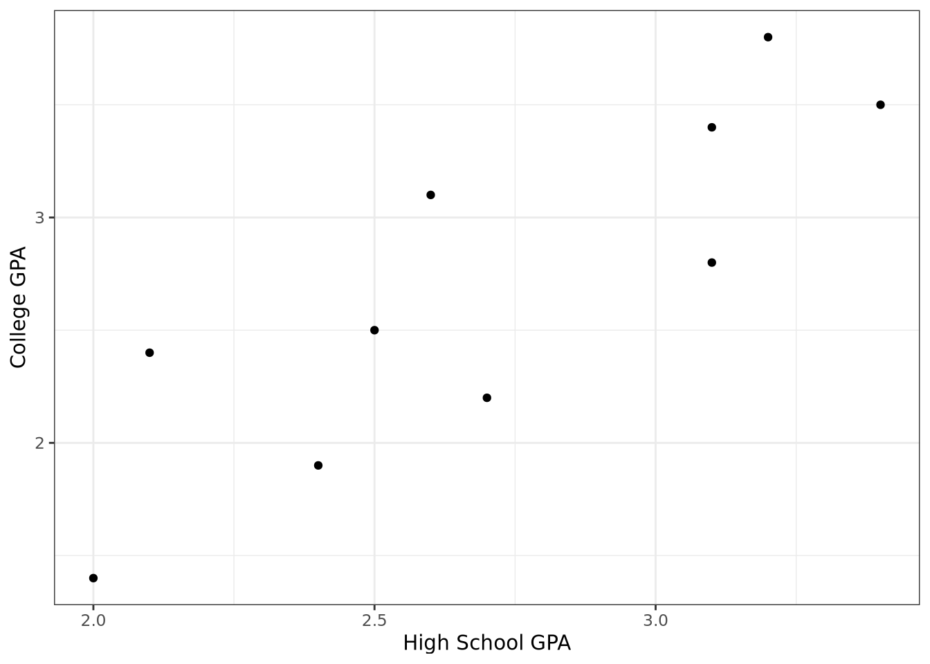
Create a scatterplot and then comment on the relationship between the two variables.
library (tidyverse)library (BSDA)ggplot (data = Gpa, aes (x = hsgpa, y = collgpa)) + labs (x = "High School GPA" , y = "College GPA" ) + geom_point () + theme_bw ()
The college GPA is the response variable and is labeled on the vertical axis. The scatterplot in Figure 1 shows that the college GPA increases as the high school GPA increases. In fact, the the dots appear to cluster along a straight line. The correlation coefficient is \(r = 0.844\) , which indicates that a straight line is a reasonable relationship between the two variables.
Compute the correlation coefficient using Equation 1 .
# A tibble: 6 × 2
  hsgpa collgpa
  <dbl>   <dbl>
1   2.7     2.2
2   3.1     2.8
3   2.1     2.4
4   3.2     3.8
5   2.4     1.9
6   3.4     3.5
<- Gpa |> mutate (y_ybar = collgpa - mean (collgpa), x_xbar = hsgpa - mean (hsgpa), zx = x_xbar/ sd (hsgpa), zy = y_ybar/ sd (collgpa),zxzy = zx* zy):: kable (values)
2.7
2.2
-0.5
-0.01
-0.0209580
-0.6565322
0.0137596
3.1
2.8
0.1
0.39
0.8173628
0.1313064
0.1073250
2.1
2.4
-0.3
-0.61
-1.2784393
-0.3939193
0.5036019
3.2
3.8
1.1
0.49
1.0269430
1.4443708
1.4832865
2.4
1.9
-0.8
-0.31
-0.6496987
-1.0504515
0.6824769
3.4
3.5
0.8
0.69
1.4461035
1.0504515
1.5190615
2.6
3.1
0.4
-0.11
-0.2305382
0.5252257
-0.1210846
2.0
1.4
-1.3
-0.71
-1.4880195
-1.7069836
2.5400249
3.1
3.4
0.7
0.39
0.8173628
0.9191450
0.7512750
2.5
2.5
-0.2
-0.21
-0.4401184
-0.2626129
0.1155808
# |> summarize (r = (1 / 9 )* sum (zxzy))
# A tibble: 1 × 1
      r
  <dbl>
1 0.844
Using the build in cor() function:
|> summarize (r = cor (collgpa, hsgpa))
# A tibble: 1 × 1
      r
  <dbl>
1 0.844
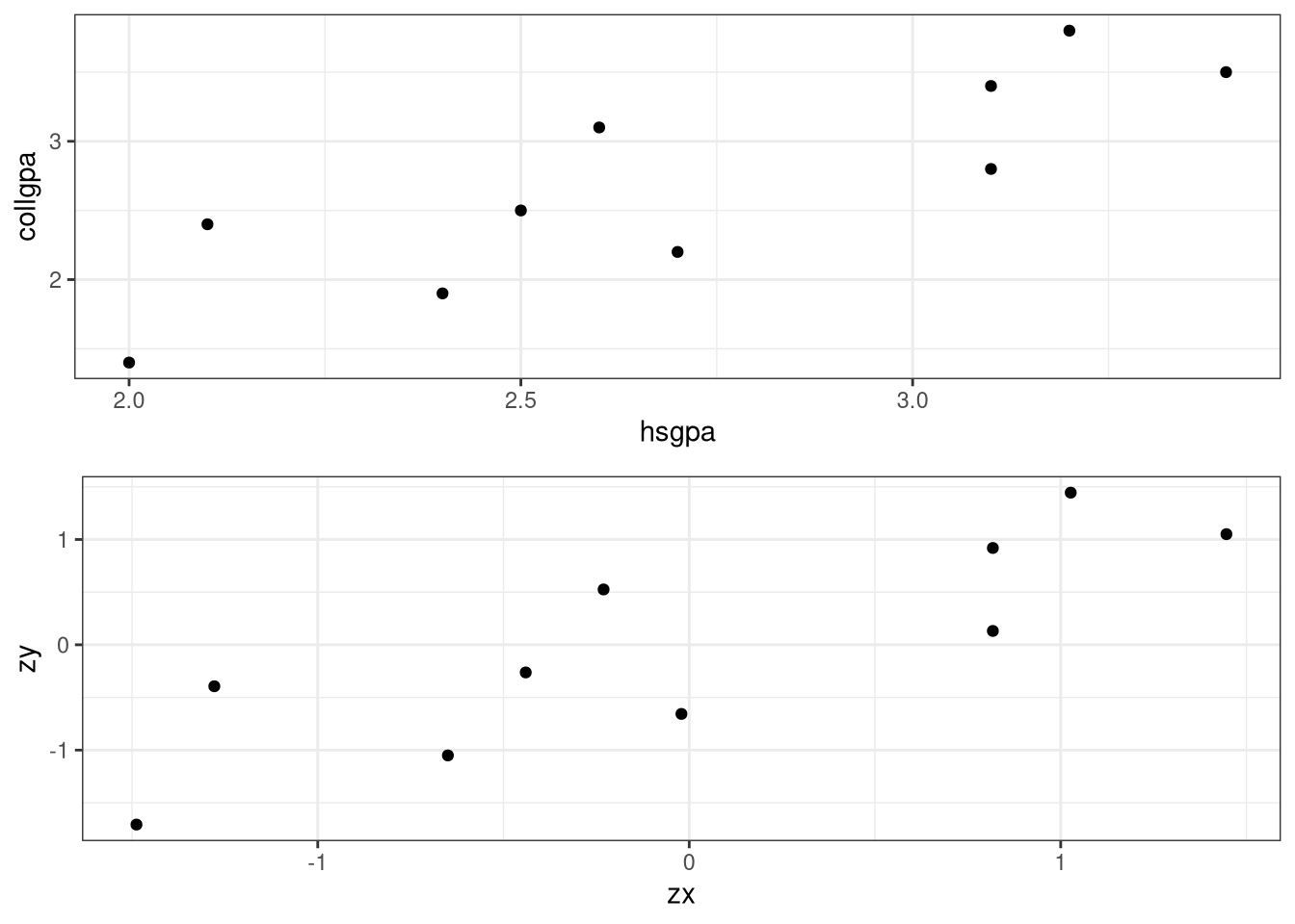
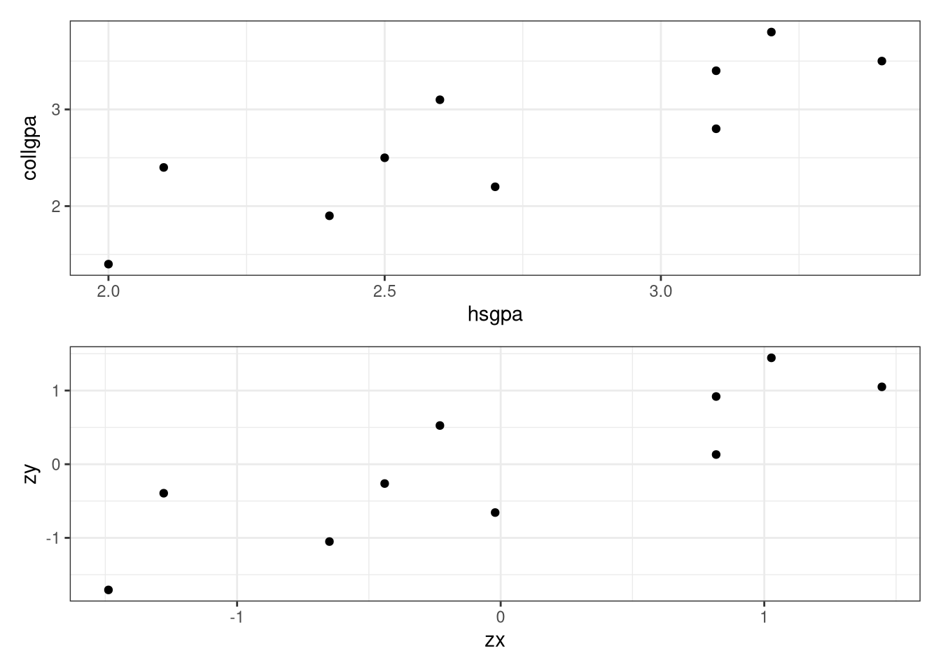
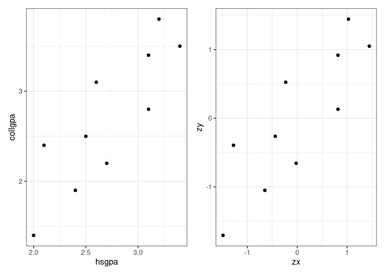
Note:
<- ggplot (data = Gpa, aes (x = hsgpa, y = collgpa)) + geom_point () + theme_bw ()<- ggplot (data = values, aes (x = zx, y = zy)) + geom_point () + theme_bw ()library (gridExtra)grid.arrange (p1, p2, ncol = 1 , nrow = 2 )# Or better yet library (patchwork)/ p2
Least Squares Regression
The equation of a straight line is
\[y = b_0 + b_1x \tag{2}\]
where \(b_0\) is the \(y\) -intercept and \(b_1\) is the slope of the line. From the equation of the line that best fits the data,
\[\hat{y} = b_0 + b_1x \tag{3}\]
we can compute a predicted \(y\) for each value of \(x\) and then measure the error of the prediction. The error of the prediction, \(e_i\) (also called the residual) is the difference in the actual \(y_i\) and the predicted \(\hat{y}_i\) . That is, the residual associated with the data point \((x_i, y_i)\) is
\[e_i = y_i - \hat{y}_i. \tag{4}\]
The least squares regression line is
\[\hat{y} = b_0 + b_1x \tag{5}\]
where
\[
b_1 = \frac{\sum(x_i - \bar{x})(y_i - \bar{y})}{\sum(x_i - \bar{x})^2} = r\frac{s_y}{s_x}
\tag{6}\]
and
\[
b_0 = \bar{y} - b_1\bar{x}
\tag{7}\]
Find the least squares regression line \(\hat{y} = b_0 + b_1x\) for the Gpa data.
|> summarize (b1 = cor (hsgpa, collgpa)* sd (collgpa)/ sd (hsgpa),b0 = mean (collgpa) - b1* mean (hsgpa)) -> ans1|> :: kable ()
\[
\widehat{\text{collgpa}} = -0.950366 + 1.3469985 \times \text{hsgpa}
\tag{8}\]
The coefficients are also computed when using the lm() function.
<- lm (collgpa ~ hsgpa, data = Gpa)
Call:
lm(formula = collgpa ~ hsgpa, data = Gpa)

Coefficients:
(Intercept)        hsgpa
    -0.9504       1.3470
Call:
lm(formula = collgpa ~ hsgpa, data = Gpa)

Residuals:
     Min       1Q   Median       3Q      Max
-0.48653 -0.37273 -0.02328  0.37365  0.54817

Coefficients:
            Estimate Std. Error t value Pr(>|t|)
(Intercept)  -0.9504     0.8318  -1.143  0.28625
hsgpa         1.3470     0.3027   4.449  0.00214 **
---
Signif. codes:  0 '***' 0.001 '**' 0.01 '*' 0.05 '.' 0.1 ' ' 1

Residual standard error: 0.4333 on 8 degrees of freedom
Multiple R-squared:  0.7122,    Adjusted R-squared:  0.6762
F-statistic:  19.8 on 1 and 8 DF,  p-value: 0.002141
\[
\widehat{\text{collgpa}} = -0.950366 + 1.3469985 \times \text{hsgpa}
\tag{9}\]
Or
\[
\widehat{\text{collgpa}} = -0.950366 + 1.3469985 \times \text{hsgpa}
\tag{10}\]
:: kable (summary (mod1)$ coef)
(Intercept)
-0.950366
0.8317729
-1.142579
0.2862536
hsgpa
1.346998
0.3027332
4.449458
0.0021408
library (moderndive)get_regression_table (mod1)
# A tibble: 2 × 7
  term      estimate std_error statistic p_value lower_ci upper_ci
  <chr>        <dbl>     <dbl>     <dbl>   <dbl>    <dbl>    <dbl>
1 intercept    -0.95     0.832     -1.14   0.286   -2.87     0.968
2 hsgpa         1.35     0.303      4.45   0.002    0.649    2.04
# Spruce up some get_regression_table (mod1) |> :: kable ()
intercept
-0.950
0.832
-1.143
0.286
-2.868
0.968
hsgpa
1.347
0.303
4.449
0.002
0.649
2.045
\[
\widehat{\text{collgpa}} = -0.95 + 1.347 \times \text{hsgpa}
\tag{11}\]
:: tidy (mod1, conf.int = TRUE ) |> :: kable ()
(Intercept)
-0.950366
0.8317729
-1.142579
0.2862536
-2.8684378
0.9677057
hsgpa
1.346998
0.3027332
4.449458
0.0021408
0.6488945
2.0451026
# GOF measures :: glance (mod1) |> :: kable ()
0.7122061
0.6762319
0.4333422
19.79767
0.0021408
1
-4.711393
15.42279
16.33054
1.502284
8
10
\[
\widehat{\text{collgpa}} = -0.950366 + 1.3469985 \times \text{hsgpa}
\tag{12}\]
Find the residuals for mod1.
get_regression_points (mod1)
# A tibble: 10 × 5
      ID collgpa hsgpa collgpa_hat residual
   <int>   <dbl> <dbl>       <dbl>    <dbl>
 1     1     2.2   2.7        2.69   -0.487
 2     2     2.8   3.1        3.22   -0.425
 3     3     2.4   2.1        1.88    0.522
 4     4     3.8   3.2        3.36    0.44
 5     5     1.9   2.4        2.28   -0.382
 6     6     3.5   3.4        3.63   -0.129
 7     7     3.1   2.6        2.55    0.548
 8     8     1.4   2          1.74   -0.344
 9     9     3.4   3.1        3.22    0.175
10    10     2.5   2.5        2.42    0.083
# Spruced up get_regression_points (mod1) |> :: kable ()
1
2.2
2.7
2.687
-0.487
2
2.8
3.1
3.225
-0.425
3
2.4
2.1
1.878
0.522
4
3.8
3.2
3.360
0.440
5
1.9
2.4
2.282
-0.382
6
3.5
3.4
3.629
-0.129
7
3.1
2.6
2.552
0.548
8
1.4
2.0
1.744
-0.344
9
3.4
3.1
3.225
0.175
10
2.5
2.5
2.417
0.083
# or broom :: augment (mod1)
# A tibble: 10 × 8
   collgpa hsgpa .fitted  .resid  .hat .sigma .cooksd .std.resid
     <dbl> <dbl>   <dbl>   <dbl> <dbl>  <dbl>   <dbl>      <dbl>
 1     2.2   2.7    2.69 -0.487  0.100  0.421 0.0779      -1.18
 2     2.8   3.1    3.23 -0.425  0.174  0.428 0.123       -1.08
 3     2.4   2.1    1.88  0.522  0.282  0.401 0.395        1.42
 4     3.8   3.2    3.36  0.440  0.217  0.423 0.183        1.15
 5     1.9   2.4    2.28 -0.382  0.147  0.436 0.0786      -0.955
 6     3.5   3.4    3.63 -0.129  0.332  0.459 0.0333      -0.366
 7     3.1   2.6    2.55  0.548  0.106  0.408 0.106        1.34
 8     1.4   2      1.74 -0.344  0.346  0.435 0.254       -0.981
 9     3.4   3.1    3.23  0.175  0.174  0.458 0.0208       0.444
10     2.5   2.5    2.42  0.0829 0.122  0.462 0.00288      0.204
# Spruced up :: augment (mod1) |> :: kable ()
2.2
2.7
2.686530
-0.4865300
0.1000488
0.4207573
0.0778576
-1.1835024
2.8
3.1
3.225329
-0.4253294
0.1742313
0.4281537
0.1230746
-1.0801031
2.4
2.1
1.878331
0.5216691
0.2816008
0.4006194
0.3953669
1.4203035
3.8
3.2
3.360029
0.4399707
0.2171791
0.4234225
0.1826622
1.1475234
1.9
2.4
2.282430
-0.3824305
0.1469009
0.4360286
0.0786029
-0.9554802
3.5
3.4
3.629429
-0.1294290
0.3323572
0.4593774
0.0332574
-0.3655346
3.1
2.6
2.551830
0.5481698
0.1059053
0.4081668
0.1059959
1.3378036
1.4
2.0
1.743631
-0.3436310
0.3460224
0.4345316
0.2543732
-0.9805730
3.4
3.1
3.225329
0.1746706
0.1742313
0.4575302
0.0207566
0.4435673
2.5
2.5
2.417130
0.0828697
0.1215227
0.4620554
0.0028794
0.2040325
Add the least squares line to the scatterplot for collgpa versus hsgpa.
ggplot (data = Gpa, aes (x = hsgpa, y = collgpa)) + geom_point () + geom_smooth (method = "lm" , se = FALSE ) + labs (x = "High School GPA" , y = "College GPA" ) + theme_bw ()
Using the model to predict
What does the least squares regression model (mod1) predict for collgpa for a student with a 3.3 hsgpa?
$ coef[1 ] + mod1$ coef[2 ]* 3.3 predict (mod1, newdata = tibble (hsgpa = 3.3 ))get_regression_points (mod1, newdata = tibble (hsgpa = 3.3 ), digits = 7 ) -> T3
# A tibble: 1 × 3
     ID hsgpa collgpa_hat
  <int> <dbl>       <dbl>
1     1   3.3        3.49
# A tibble: 1 × 1
  collgpa_hat
        <dbl>
1        3.49
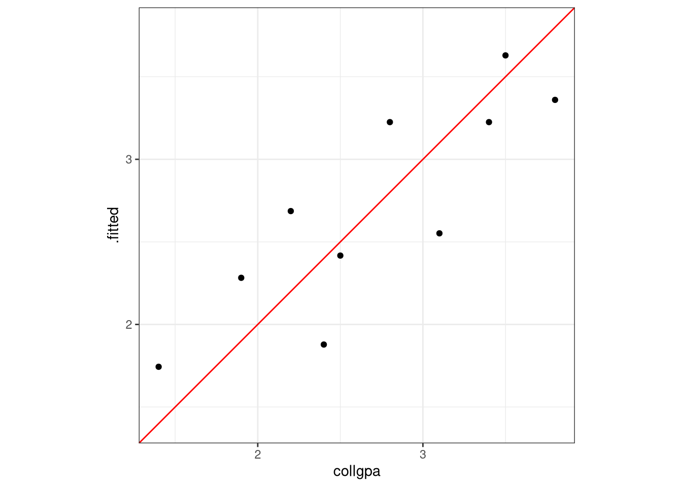
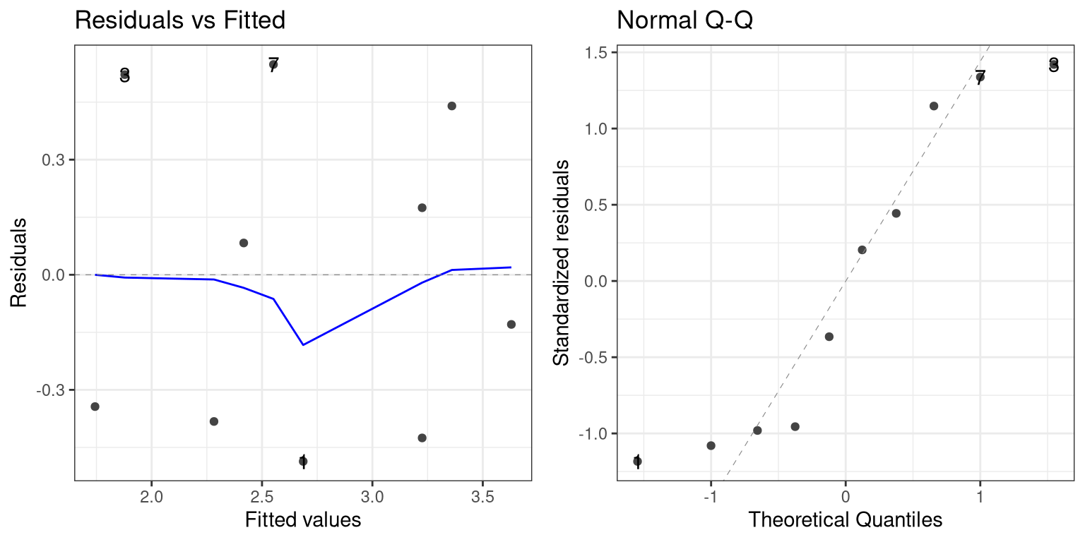
Assessing the fit
# R^2 plot :: augment (mod1) |> ggplot (aes (x = collgpa, y = .fitted)) + geom_point () + geom_abline (color = "red" ) + :: coord_obs_pred () + theme_bw ()
library (ggfortify)autoplot (mod1, ncol = 2 , nrow = 1 , which = 1 : 2 ) + theme_bw ()