Chapter 4 Data Manipulation using dplyr and tidyr
Learning Objectives
- Describe the purpose of the
dplyrand thetidyrpackages written by (Wickham, François, et al. 2020) and (Wickham and Henry 2020), respectively. - Select certain columns in a data frame with the
dplyrfunctionselect. - Select certain rows in a data frame according to filtering conditions with the
dplyrfunctionfilter. - Link the output of one
dplyrfunction to the input of another function with the ‘pipe’ operator%>%. - Add new columns to a data frame that are functions of existing columns with
mutate. - Use the split-apply-combine concept for data analysis.
- Use
summarize,group_by, andcountto split a data frame into groups of observations, apply summary statistics for each group, and then combine the results. - Describe the concept of a wide and a long table format and for which purpose those formats are useful.
- Describe what key-value pairs are.
- Reshape a data frame from long to wide format and back with the
pivot_widerandpivot_longercommands from thetidyrpackage. - Export a data frame to a .csv file.
Bracket subsetting is handy, but it can be cumbersome and difficult to read, especially for complicated operations. Enter dplyr. dplyr is a package for making tabular data manipulation easier. It pairs nicely with tidyr which enables you to swiftly convert between different data formats for plotting and analysis.
Packages in R are basically sets of additional functions that let you do more stuff. The functions we’ve been using so far, like str() or data.frame(), come built into R; packages give you access to more of them. Before you use a package for the first time you need to install it on your machine, and then you should import it in every subsequent R session when you need it. You should already have installed the tidyverse package written by (Wickham 2019). This is an “umbrella-package” that installs several packages useful for data analysis which work together well such as tidyr, dplyr, ggplot2, tibble, etc.
The tidyverse package tries to address 3 common issues that arise when doing data analysis with some of the functions that come with R:
- The results from a base R function sometimes depend on the type of data.
- Using R expressions in a non standard way, which can be confusing for new learners.
- Hidden arguments, having default operations that new learners are not aware of.
We have seen in our previous lesson that when building or importing a data frame, the columns that contain characters (i.e., text) are coerced (=converted) into the factor data type. We had to set stringsAsFactors to FALSE to avoid this hidden argument to convert our data type.
This time we will use the tidyverse package to read the data and avoid having to set stringsAsFactors to FALSE
If we haven’t already done so, we can type install.packages("tidyverse") straight into the console. In fact, it’s better to write this in the console than in our script for any package, as there’s no need to re-install packages every time we run the script.
Then, to load the package type:
## load the tidyverse packages, incl. dplyr
library(tidyverse)
4.1 What are dplyr and tidyr?
The package dplyr provides easy tools for the most common data manipulation tasks. It is built to work directly with data frames, with many common tasks optimized by being written in a compiled language (C++). An additional feature is the ability to work directly with data stored in an external database. The benefits of doing this are that the data can be managed natively in a relational database, queries can be conducted on that database, and only the results of the query are returned.
This addresses a common problem with R in that all operations are conducted in-memory and thus the amount of data you can work with is limited by available memory. The database connections essentially remove that limitation in that you can connect to a database of many hundreds of GB, conduct queries on it directly, and pull back into R only what you need for analysis.
The package tidyr addresses the common problem of wanting to reshape your data for plotting and use by different R functions. Sometimes we want data sets where we have one row per measurement. Sometimes we want a data frame where each measurement type has its own column, and rows are instead more aggregated groups - like plots or aquaria. Moving back and forth between these formats is non-trivial, and tidyr gives you tools for this and more sophisticated data manipulation.
To learn more about dplyr and tidyr after the workshop, you may want to check out this handy data transformation with dplyr cheatsheet and this one about tidyr.
We’ll read in our data using the read_csv() function, from the tidyverse package readr, instead of using the base R read.csv() function.
surveys <- read_csv("data_raw/portal_data_joined.csv")You will see the message Parsed with column specification, followed by each column name and its data type. When you execute read_csv on a data file, it looks through the first 1000 rows of each column and guesses the data type for each column as it reads it into R. For example, in this dataset, read_csv reads weight as col_double (a numeric data type), and species as col_character. You have the option to specify the data type for a column manually by using the col_types argument in read_csv.
## inspect the data
str(surveys)
tibble [34,786 × 13] (S3: spec_tbl_df/tbl_df/tbl/data.frame)
$ record_id : num [1:34786] 1 72 224 266 349 363 435 506 588 661 ...
$ month : num [1:34786] 7 8 9 10 11 11 12 1 2 3 ...
$ day : num [1:34786] 16 19 13 16 12 12 10 8 18 11 ...
$ year : num [1:34786] 1977 1977 1977 1977 1977 ...
$ plot_id : num [1:34786] 2 2 2 2 2 2 2 2 2 2 ...
$ species_id : chr [1:34786] "NL" "NL" "NL" "NL" ...
$ sex : chr [1:34786] "M" "M" NA NA ...
$ hindfoot_length: num [1:34786] 32 31 NA NA NA NA NA NA NA NA ...
$ weight : num [1:34786] NA NA NA NA NA NA NA NA 218 NA ...
$ genus : chr [1:34786] "Neotoma" "Neotoma" "Neotoma" "Neotoma" ...
$ species : chr [1:34786] "albigula" "albigula" "albigula" "albigula" ...
$ taxa : chr [1:34786] "Rodent" "Rodent" "Rodent" "Rodent" ...
$ plot_type : chr [1:34786] "Control" "Control" "Control" "Control" ...
- attr(*, "spec")=
.. cols(
.. record_id = col_double(),
.. month = col_double(),
.. day = col_double(),
.. year = col_double(),
.. plot_id = col_double(),
.. species_id = col_character(),
.. sex = col_character(),
.. hindfoot_length = col_double(),
.. weight = col_double(),
.. genus = col_character(),
.. species = col_character(),
.. taxa = col_character(),
.. plot_type = col_character()
.. )## preview the data
View(surveys)Notice that the class of the data is now tbl
This is referred to as a “tibble”. Tibbles tweak some of the behaviors of the data frame objects we introduced in the previous episode. The data structure is very similar to a data frame. For our purposes the only differences are that:
- In addition to displaying the data type of each column under its name, it only prints the first few rows of data and only as many columns as fit on one screen.
- Columns of class
characterare never converted into factors.
We’re going to learn some of the most common dplyr functions:
select(): subset columnsfilter(): subset rows on conditionsmutate(): create new columns by using information from other columnsgroup_by()andsummarize(): create summary statistics on grouped dataarrange(): sort resultscount(): count discrete values
4.2 Selecting columns and filtering rows
To select columns of a data frame, use select(). The first argument to this function is the data frame (surveys), and the subsequent arguments are the columns to keep.
select(surveys, plot_id, species_id, weight) %>%
  head()
# A tibble: 6 x 3
plot_id species_id weight
<dbl> <chr> <dbl>
1 2 NL NA
2 2 NL NA
3 2 NL NA
4 2 NL NA
5 2 NL NA
6 2 NL NA# Or
surveys %>%
select(plot_id, species_id, weight) %>%
head()# A tibble: 6 x 3
plot_id species_id weight
<dbl> <chr> <dbl>
1 2 NL NA
2 2 NL NA
3 2 NL NA
4 2 NL NA
5 2 NL NA
6 2 NL NATo select all columns except certain ones, put a “-” in front of the variable to exclude it.
select(surveys, -record_id, -species_id) %>%
  head()
# A tibble: 6 x 11
month day year plot_id sex hindfoot_length weight genus species taxa
<dbl> <dbl> <dbl> <dbl> <chr> <dbl> <dbl> <chr> <chr> <chr>
1 7 16 1977 2 M 32 NA Neot… albigu… Rode…
2 8 19 1977 2 M 31 NA Neot… albigu… Rode…
3 9 13 1977 2 <NA> NA NA Neot… albigu… Rode…
4 10 16 1977 2 <NA> NA NA Neot… albigu… Rode…
5 11 12 1977 2 <NA> NA NA Neot… albigu… Rode…
6 11 12 1977 2 <NA> NA NA Neot… albigu… Rode…
# … with 1 more variable: plot_type <chr># Or
surveys %>%
select(-record_id, -species_id) %>%
head()# A tibble: 6 x 11
month day year plot_id sex hindfoot_length weight genus species taxa
<dbl> <dbl> <dbl> <dbl> <chr> <dbl> <dbl> <chr> <chr> <chr>
1 7 16 1977 2 M 32 NA Neot… albigu… Rode…
2 8 19 1977 2 M 31 NA Neot… albigu… Rode…
3 9 13 1977 2 <NA> NA NA Neot… albigu… Rode…
4 10 16 1977 2 <NA> NA NA Neot… albigu… Rode…
5 11 12 1977 2 <NA> NA NA Neot… albigu… Rode…
6 11 12 1977 2 <NA> NA NA Neot… albigu… Rode…
# … with 1 more variable: plot_type <chr>This will select all the variables in surveys except record_id and species_id.
To choose rows based on a specific criterion, use filter():
filter(surveys, year == 1995) %>%
  head()
# A tibble: 6 x 13
record_id month day year plot_id species_id sex hindfoot_length weight
<dbl> <dbl> <dbl> <dbl> <dbl> <chr> <chr> <dbl> <dbl>
1 22314 6 7 1995 2 NL M 34 NA
2 22728 9 23 1995 2 NL F 32 165
3 22899 10 28 1995 2 NL F 32 171
4 23032 12 2 1995 2 NL F 33 NA
5 22003 1 11 1995 2 DM M 37 41
6 22042 2 4 1995 2 DM F 36 45
# … with 4 more variables: genus <chr>, species <chr>, taxa <chr>,
# plot_type <chr># Or
surveys %>%
filter(year == 1995) %>%
head()# A tibble: 6 x 13
record_id month day year plot_id species_id sex hindfoot_length weight
<dbl> <dbl> <dbl> <dbl> <dbl> <chr> <chr> <dbl> <dbl>
1 22314 6 7 1995 2 NL M 34 NA
2 22728 9 23 1995 2 NL F 32 165
3 22899 10 28 1995 2 NL F 32 171
4 23032 12 2 1995 2 NL F 33 NA
5 22003 1 11 1995 2 DM M 37 41
6 22042 2 4 1995 2 DM F 36 45
# … with 4 more variables: genus <chr>, species <chr>, taxa <chr>,
# plot_type <chr>4.3 Pipes
What if you want to select and filter at the same time? There are three ways to do this: use intermediate steps, nested functions, or pipes.
With intermediate steps, you create a temporary data frame and use that as input to the next function, like this:
surveys2 <- filter(surveys, weight < 5)
surveys_sml <- select(surveys2, species_id, sex, weight)
head(surveys_sml)
# A tibble: 6 x 3
species_id sex weight
<chr> <chr> <dbl>
1 PF F 4
2 PF F 4
3 PF M 4
4 RM F 4
5 RM M 4
6 PF <NA> 4This is readable, but can clutter up your workspace with lots of objects that you have to name individually. With multiple steps, that can be hard to keep track of.
You can also nest functions (i.e. one function inside of another), like this:
surveys_sml <- select(filter(surveys, weight < 5), species_id, sex, weight)
head(surveys_sml)
# A tibble: 6 x 3
species_id sex weight
<chr> <chr> <dbl>
1 PF F 4
2 PF F 4
3 PF M 4
4 RM F 4
5 RM M 4
6 PF <NA> 4This is handy, but can be difficult to read if too many functions are nested, as R evaluates the expression from the inside out (in this case, filtering, then selecting).
The last option, pipes, are a recent addition to R. Pipes let you take the output of one function and send it directly to the next, which is useful when you need to do many things to the same dataset. Pipes in R look like %>% and are made available via the magrittr package written by (Bache and Wickham 2014), which is installed automatically with dplyr. If you use RStudio, you can type the pipe with Ctrl + Shift + M if you have a PC or Cmd + Shift + M if you have a Mac.
surveys %>%
  filter(weight < 5) %>%
  select(species_id, sex, weight) %>%
  head()
# A tibble: 6 x 3
species_id sex weight
<chr> <chr> <dbl>
1 PF F 4
2 PF F 4
3 PF M 4
4 RM F 4
5 RM M 4
6 PF <NA> 4In the above code, we use the pipe to send the surveys dataset first through filter() to keep rows where weight is less than 5, then through select() to keep only the species_id, sex, and weight columns. Since %>% takes the object on its left and passes it as the first argument to the function on its right, we don’t need to explicitly include the data frame as an argument to the filter() and select() functions any more.
Some may find it helpful to read the pipe like the word “then”. For instance, in the above example, we took the data frame surveys, then we filtered for rows with weight < 5, then we selected columns species_id, sex, and weight. The dplyr functions by themselves are somewhat simple, but by combining them into linear workflows with the pipe, we can accomplish more complex manipulations of data frames.
If we want to create a new object with this smaller version of the data, we can assign it a new name:
surveys_sml <- surveys %>%
  filter(weight < 5) %>%
  select(species_id, sex, weight)
surveys_sml %>%
  head()
# A tibble: 6 x 3
species_id sex weight
<chr> <chr> <dbl>
1 PF F 4
2 PF F 4
3 PF M 4
4 RM F 4
5 RM M 4
6 PF <NA> 4Note that the final data frame is the leftmost part of this expression.
Challenge
- Using pipes, subset the
surveysdata to include animals collected before 1995 and retain only the columnsyear,sex, andweight.
Solution
4.4 Mutate
Frequently you’ll want to create new columns based on the values in existing columns, for example to do unit conversions, or to find the ratio of values in two columns. For this we’ll use mutate().
To create a new column of weight in kg:
surveys %>%
  mutate(weight_kg = weight / 1000) %>%
  select(weight, weight_kg)
# A tibble: 34,786 x 2
weight weight_kg
<dbl> <dbl>
1 NA NA
2 NA NA
3 NA NA
4 NA NA
5 NA NA
6 NA NA
7 NA NA
8 NA NA
9 218 0.218
10 NA NA
# … with 34,776 more rowsYou can also create a second new column based on the first new column within the same call of mutate():
surveys %>%
  mutate(weight_kg = weight / 1000,
         weight_lb = weight_kg * 2.2) %>%
  select(weight, weight_kg, weight_lb)
# A tibble: 34,786 x 3
weight weight_kg weight_lb
<dbl> <dbl> <dbl>
1 NA NA NA
2 NA NA NA
3 NA NA NA
4 NA NA NA
5 NA NA NA
6 NA NA NA
7 NA NA NA
8 NA NA NA
9 218 0.218 0.480
10 NA NA NA
# … with 34,776 more rowsIf this runs off your screen and you just want to see the first few rows, you can use a pipe to view the head() of the data. (Pipes work with non-dplyr functions, too, as long as the dplyr or magrittr package is loaded).
surveys %>%
  mutate(weight_kg = weight / 1000) %>%
  select(weight, weight_kg) %>%
  head()
# A tibble: 6 x 2
weight weight_kg
<dbl> <dbl>
1 NA NA
2 NA NA
3 NA NA
4 NA NA
5 NA NA
6 NA NAThe first few rows of the output are full of NAs, so if we wanted to remove those we could insert a filter() in the chain:
surveys %>%
  filter(!is.na(weight)) %>%
  mutate(weight_kg = weight / 1000) %>%
  select(weight:weight_kg) %>%
  head()
# A tibble: 6 x 6
weight genus species taxa plot_type weight_kg
<dbl> <chr> <chr> <chr> <chr> <dbl>
1 218 Neotoma albigula Rodent Control 0.218
2 204 Neotoma albigula Rodent Control 0.204
3 200 Neotoma albigula Rodent Control 0.2
4 199 Neotoma albigula Rodent Control 0.199
5 197 Neotoma albigula Rodent Control 0.197
6 218 Neotoma albigula Rodent Control 0.218is.na() is a function that determines whether something is an NA. The ! symbol negates the result, so we’re asking for every row where weight is not an NA.
Challenge
Create a new data frame from the surveys data that meets the following criteria: contains only the species_id column and a new column called hindfoot_cm containing the hindfoot_length values converted to centimeters. In this hindfoot_cm column, there are no NAs and all values are less than 3.
Hint: think about how the commands should be ordered to produce this data frame!
Solution
4.5 Split-apply-combine data analysis and the summarize() function
Many data analysis tasks can be approached using the split-apply-combine paradigm: split the data into groups, apply some analysis to each group, and then combine the results. dplyr makes this very easy through the use of the group_by() function.
4.5.1 The summarize() function
group_by() is often used together with summarize(), which collapses each group into a single-row summary of that group. group_by() takes as arguments the column names that contain the categorical variables for which you want to calculate the summary statistics. So to compute the mean weight by sex:
surveys %>%
  group_by(sex) %>%
  summarize(mean_weight = mean(weight, na.rm = TRUE))
# A tibble: 3 x 2
sex mean_weight
<chr> <dbl>
1 F 42.2
2 M 43.0
3 <NA> 64.7You may also have noticed that the output from these calls doesn’t run off the screen anymore. It’s one of the advantages of tbl_df over data frame.
You can also group by multiple columns:
surveys %>%
  group_by(sex, species_id) %>%
  summarize(mean_weight = mean(weight, na.rm = TRUE)) %>%
  head()
# A tibble: 6 x 3
# Groups: sex [1]
sex species_id mean_weight
<chr> <chr> <dbl>
1 F BA 9.16
2 F DM 41.6
3 F DO 48.5
4 F DS 118.
5 F NL 154.
6 F OL 31.1 ####
surveys %>%
group_by(sex, species_id) %>%
summarize(mean_weight = mean(weight, na.rm = TRUE)) %>%
tail()# A tibble: 6 x 3
# Groups: sex [1]
sex species_id mean_weight
<chr> <chr> <dbl>
1 <NA> SU NaN
2 <NA> UL NaN
3 <NA> UP NaN
4 <NA> UR NaN
5 <NA> US NaN
6 <NA> ZL NaNWhen grouping both by sex and species_id, the last few rows are for animals that escaped before their sex and body weights could be determined. You may notice that the last column does not contain NA but NaN (which refers to “Not a Number”). To avoid this, we can remove the missing values for weight before we attempt to calculate the summary statistics on weight. Because the missing values are removed first, we can omit na.rm = TRUE when computing the mean:
surveys %>%
  filter(!is.na(weight)) %>%
  group_by(sex, species_id) %>%
  summarize(mean_weight = mean(weight))
# A tibble: 64 x 3
# Groups: sex [3]
sex species_id mean_weight
<chr> <chr> <dbl>
1 F BA 9.16
2 F DM 41.6
3 F DO 48.5
4 F DS 118.
5 F NL 154.
6 F OL 31.1
7 F OT 24.8
8 F OX 21
9 F PB 30.2
10 F PE 22.8
# … with 54 more rowsHere, again, the output from these calls doesn’t run off the screen anymore. If you want to display more data, you can use the print() function at the end of your chain with the argument n specifying the number of rows to display:
surveys %>%
  filter(!is.na(weight)) %>%
  group_by(sex, species_id) %>%
  summarize(mean_weight = mean(weight)) %>%
  print(n = 15)
# A tibble: 64 x 3
# Groups: sex [3]
sex species_id mean_weight
<chr> <chr> <dbl>
1 F BA 9.16
2 F DM 41.6
3 F DO 48.5
4 F DS 118.
5 F NL 154.
6 F OL 31.1
7 F OT 24.8
8 F OX 21
9 F PB 30.2
10 F PE 22.8
11 F PF 7.97
12 F PH 30.8
13 F PL 19.3
14 F PM 22.1
15 F PP 17.2
# … with 49 more rowsOnce the data are grouped, you can also summarize multiple variables at the same time (and not necessarily on the same variable). For instance, we could add a column indicating the minimum weight for each species for each sex:
surveys %>%
  filter(!is.na(weight)) %>%
  group_by(sex, species_id) %>%
  summarize(mean_weight = mean(weight),
            min_weight = min(weight))
# A tibble: 64 x 4
# Groups: sex [3]
sex species_id mean_weight min_weight
<chr> <chr> <dbl> <dbl>
1 F BA 9.16 6
2 F DM 41.6 10
3 F DO 48.5 12
4 F DS 118. 45
5 F NL 154. 32
6 F OL 31.1 10
7 F OT 24.8 5
8 F OX 21 20
9 F PB 30.2 12
10 F PE 22.8 11
# … with 54 more rowsIt is sometimes useful to rearrange the result of a query to inspect the values. For instance, we can sort on min_weight to put the lighter species first:
surveys %>%
  filter(!is.na(weight)) %>%
  group_by(sex, species_id) %>%
  summarize(mean_weight = mean(weight),
            min_weight = min(weight)) %>%
  arrange(min_weight)
# A tibble: 64 x 4
# Groups: sex [3]
sex species_id mean_weight min_weight
<chr> <chr> <dbl> <dbl>
1 F PF 7.97 4
2 F RM 11.1 4
3 M PF 7.89 4
4 M PP 17.2 4
5 M RM 10.1 4
6 <NA> PF 6 4
7 F OT 24.8 5
8 F PP 17.2 5
9 F BA 9.16 6
10 M BA 7.36 6
# … with 54 more rowsTo sort in descending order, we need to add the desc() function. If we want to sort the results by decreasing order of mean weight:
surveys %>%
  filter(!is.na(weight)) %>%
  group_by(sex, species_id) %>%
  summarize(mean_weight = mean(weight),
            min_weight = min(weight)) %>%
  arrange(desc(mean_weight))
# A tibble: 64 x 4
# Groups: sex [3]
sex species_id mean_weight min_weight
<chr> <chr> <dbl> <dbl>
1 <NA> NL 168. 83
2 M NL 166. 30
3 F NL 154. 32
4 M SS 130 130
5 <NA> SH 130 130
6 M DS 122. 12
7 <NA> DS 120 78
8 F DS 118. 45
9 F SH 78.8 30
10 F SF 69 46
# … with 54 more rows4.5.2 Counting
When working with data, we often want to know the number of observations found for each factor or combination of factors. For this task, dplyr provides count(). For example, if we wanted to count the number of rows of data for each sex, we would do:
surveys %>%
    count(sex)
# A tibble: 3 x 2
sex n
<chr> <int>
1 F 15690
2 M 17348
3 <NA> 1748The same type of traditional cross-tabulation is accomplished in base R with table() and xtabs().
table(surveys$sex)
    F     M
15690 17348
# Or
xtabs(~sex, data = surveys)sex
F M
15690 17348 The count() function is shorthand for something we’ve already seen: grouping by a variable, and summarizing it by counting the number of observations in that group. In other words, surveys %>% count() is equivalent to:
surveys %>%
    group_by(sex) %>%
    summarise(count = n())
# A tibble: 3 x 2
sex count
<chr> <int>
1 F 15690
2 M 17348
3 <NA> 1748For convenience, count() provides the sort argument:
surveys %>%
    count(sex, sort = TRUE)
# A tibble: 3 x 2
sex n
<chr> <int>
1 M 17348
2 F 15690
3 <NA> 1748The previous example shows the use of count() to enumerate the number of rows/observations for one factor (i.e., sex). If we wanted to count a combination of factors, such as sex and species, we would specify the first and the second factor as the arguments of count():
surveys %>%
  count(sex, species)
# A tibble: 81 x 3
sex species n
<chr> <chr> <int>
1 F albigula 675
2 F baileyi 1646
3 F eremicus 579
4 F flavus 757
5 F fulvescens 57
6 F fulviventer 17
7 F hispidus 99
8 F leucogaster 475
9 F leucopus 16
10 F maniculatus 382
# … with 71 more rowsWith the above code, we can proceed with arrange() to sort the table according to a number of criteria so that we have a better comparison. For instance, we might want to arrange the table above in (i) an alphabetical order of the levels of the species and (ii) in descending order of the count:
surveys %>%
  count(sex, species) %>%
  arrange(species, desc(n))
# A tibble: 81 x 3
sex species n
<chr> <chr> <int>
1 F albigula 675
2 M albigula 502
3 <NA> albigula 75
4 <NA> audubonii 75
5 F baileyi 1646
6 M baileyi 1216
7 <NA> baileyi 29
8 <NA> bilineata 303
9 <NA> brunneicapillus 50
10 <NA> chlorurus 39
# … with 71 more rowsFrom the table above, we may learn that, for instance, there are 75 observations of the albigula species that are not specified for its sex (i.e. NA).
Challenge
How many animals were caught in each
plot_type?Use
group_by()andsummarize()to find the mean, min, and max hindfoot length for each species (usingspecies_id). Also add the number of observations (hint: see?n).What was the heaviest animal measured in each year? Return the columns
year,genus,species_id, andweight.
Solution
4.6 Reshaping with pivot_longer() and pivot_wider()
The spreadsheet lesson discusses how to structure data to satisfy the four rules defining a tidy dataset. The four rules defining a tidy dataset are:
- Each variable has its own column
- Each observation has its own row
- Each value must have its own cell
- Each type of observational unit forms a table
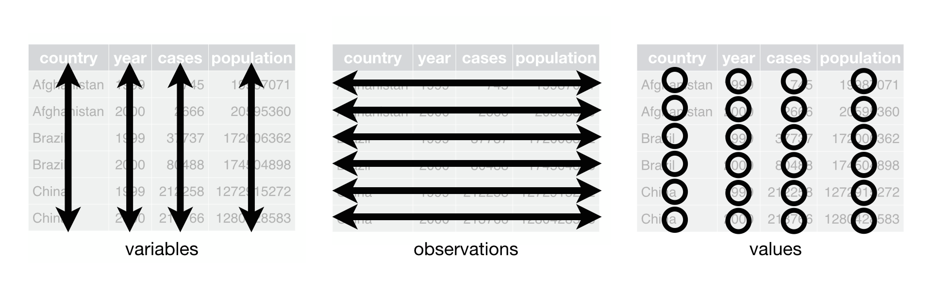
Figure 4.1: Following three rules makes a dataset tidy: variables are in columns, observations are in rows, and values are in cells.
Tidy data
Note: The Tidy data subsection material comes from R for Data Science with slight modifications.
You can represent the same underlying data in multiple ways. The example below shows the same data organized in four different ways. Each dataset shows the same values of four variables country, year, population, and cases, but each dataset organizes the values in a different way.
table1# A tibble: 6 x 4
country year cases population
<chr> <int> <int> <int>
1 Afghanistan 1999 745 19987071
2 Afghanistan 2000 2666 20595360
3 Brazil 1999 37737 172006362
4 Brazil 2000 80488 174504898
5 China 1999 212258 1272915272
6 China 2000 213766 1280428583table2# A tibble: 12 x 4
country year type count
<chr> <int> <chr> <int>
1 Afghanistan 1999 cases 745
2 Afghanistan 1999 population 19987071
3 Afghanistan 2000 cases 2666
4 Afghanistan 2000 population 20595360
5 Brazil 1999 cases 37737
6 Brazil 1999 population 172006362
7 Brazil 2000 cases 80488
8 Brazil 2000 population 174504898
9 China 1999 cases 212258
10 China 1999 population 1272915272
11 China 2000 cases 213766
12 China 2000 population 1280428583table3 # A tibble: 6 x 3
country year rate
* <chr> <int> <chr>
1 Afghanistan 1999 745/19987071
2 Afghanistan 2000 2666/20595360
3 Brazil 1999 37737/172006362
4 Brazil 2000 80488/174504898
5 China 1999 212258/1272915272
6 China 2000 213766/1280428583# Spread across two tibbles
table4a # cases# A tibble: 3 x 3
country `1999` `2000`
* <chr> <int> <int>
1 Afghanistan 745 2666
2 Brazil 37737 80488
3 China 212258 213766table4b # population# A tibble: 3 x 3
country `1999` `2000`
* <chr> <int> <int>
1 Afghanistan 19987071 20595360
2 Brazil 172006362 174504898
3 China 1272915272 1280428583These are all representations of the same underlying data, but they are not equally easy to use. One dataset, the tidy dataset (table1), will be much easier to work with inside the tidyverse.
4.6.1 Longer — Using pivot_longer()
A common problem is a dataset where some of the column names are not names of variables, but values of a variable. Take table4a; the column names 1999 and 2000 represent values of the year variable. The values in the 1999 and 2000 columns represent values of the cases variable, and each row represents two observations, not one.
table4a# A tibble: 3 x 3
country `1999` `2000`
* <chr> <int> <int>
1 Afghanistan 745 2666
2 Brazil 37737 80488
3 China 212258 213766To tidy a dataset like this, we need to gather/pivot the offending columns into a new pair of variables. To describe that operation we need three parameters:
The set of columns whose names are values, not variables. In this example, those are the columns
1999and2000.The name of the variable to move the column names to. Here it is
year.The name of the variable to move the column values to. Here it is
cases.
Together those parameters generate the call to pivot_longer():
table4a %>%
  pivot_longer(cols = c(`1999`, `2000`), names_to = "year", values_to = "cases")
# A tibble: 6 x 3
country year cases
<chr> <chr> <int>
1 Afghanistan 1999 745
2 Afghanistan 2000 2666
3 Brazil 1999 37737
4 Brazil 2000 80488
5 China 1999 212258
6 China 2000 213766The columns to gather are specified with dplyr::select() style notation. Here there are only two columns, so we list them individually. Note that “1999” and “2000” are non-syntactic names (because they don’t start with a letter) so we have to surround them in backticks. In the final result, the pivoted columns are dropped, and we get new year and cases columns. Otherwise, the relationships between the original variables are preserved. Visually, this is shown in Figure 4.2.
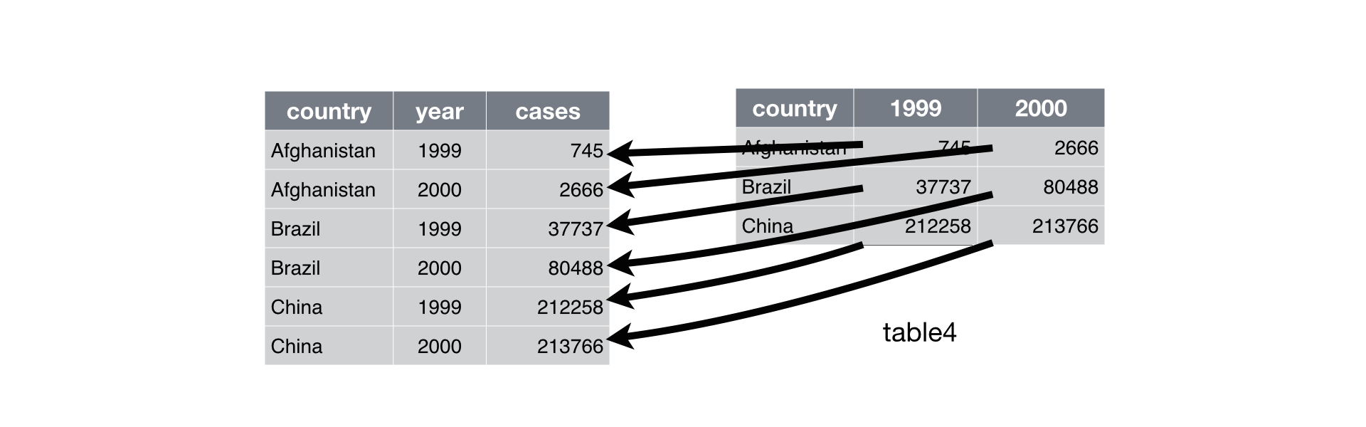
Figure 4.2: Pivoting table4 into a longer, tidy form.
pivot_longer() makes datasets longer by increasing the number of rows and decreasing the number of columns.
4.6.2 Wider — Using pivot_wider()
pivot_wider() is the opposite of pivot_longer(). You use it when an observation is scattered across multiple rows. For example, take table2: an observation is a country in a year, but each observation is spread across two rows.
table2# A tibble: 12 x 4
country year type count
<chr> <int> <chr> <int>
1 Afghanistan 1999 cases 745
2 Afghanistan 1999 population 19987071
3 Afghanistan 2000 cases 2666
4 Afghanistan 2000 population 20595360
5 Brazil 1999 cases 37737
6 Brazil 1999 population 172006362
7 Brazil 2000 cases 80488
8 Brazil 2000 population 174504898
9 China 1999 cases 212258
10 China 1999 population 1272915272
11 China 2000 cases 213766
12 China 2000 population 1280428583To tidy this up, we first analyse the representation in similar way to pivot_longer(). This time, however, we only need two parameters:
The column to take variable names from. Here it’s
type.The column that contains values from multiple variables. Here it’s
count.
Once we’ve figured that out, we can use pivot_wider(), as shown programmatically below, and visually in Figure 4.3.
table2 %>%
    pivot_wider(names_from = type, values_from = count)
# A tibble: 6 x 4
country year cases population
<chr> <int> <int> <int>
1 Afghanistan 1999 745 19987071
2 Afghanistan 2000 2666 20595360
3 Brazil 1999 37737 172006362
4 Brazil 2000 80488 174504898
5 China 1999 212258 1272915272
6 China 2000 213766 1280428583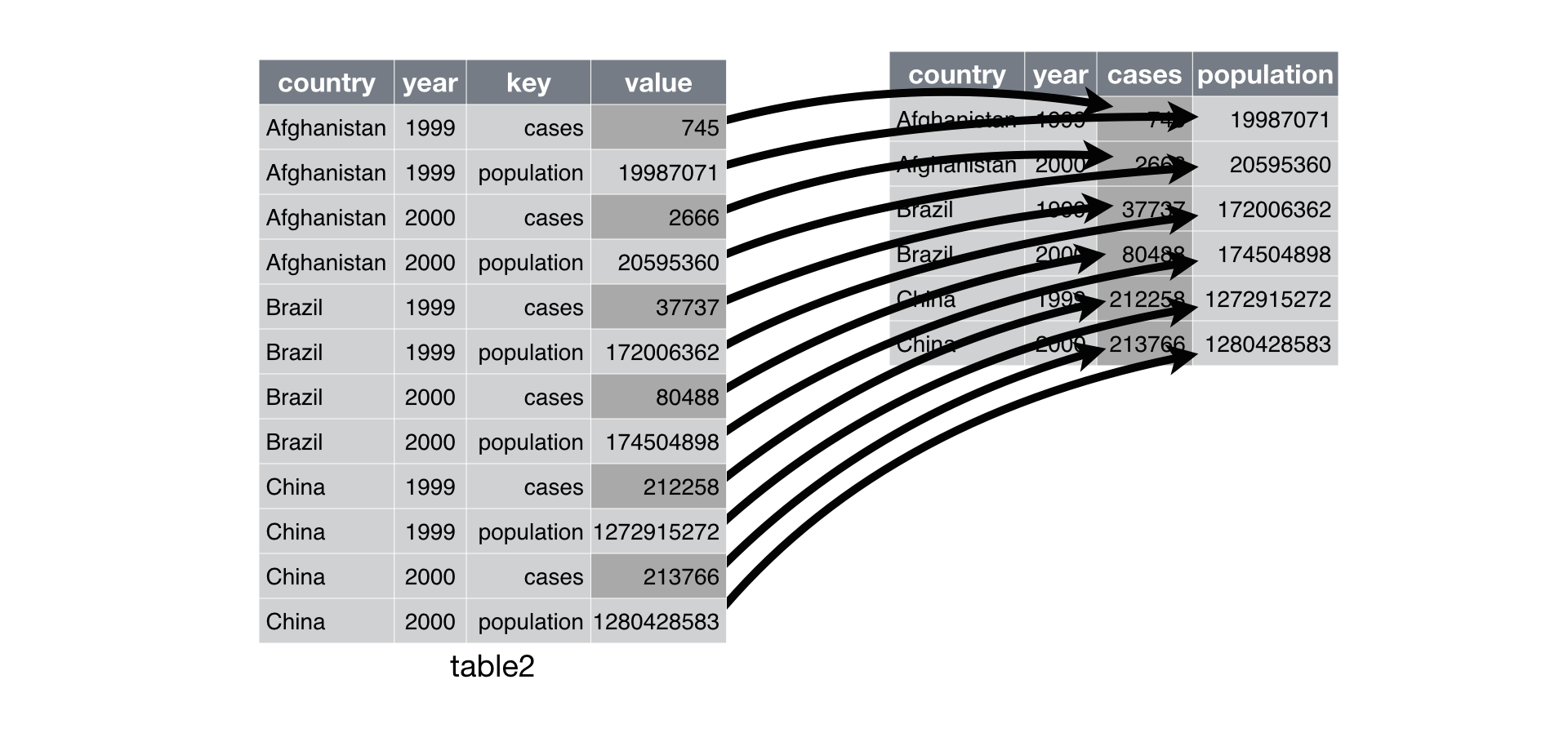
Figure 4.3: Spreading table2 makes it tidy
As you might have guessed from their names, pivot_wider() and pivot_longer() are complements. pivot_longer() makes wide tables narrower and longer; pivot_wider() makes long tables shorter and wider.
Here we examine the fourth rule: Each type of observational unit forms a table.
In surveys, the rows of surveys contain the values of variables associated with each record (the unit), values such as the weight or sex of each animal associated with each record. What if instead of comparing records, we wanted to compare the different mean weight of each genus between plots (plot_id)? (Ignoring plot_type for simplicity).
We’d need to create a new table where each row (the unit) is comprised of values of variables associated with each plot (plot_id). In practical terms this means the values in genus would become the names of column variables and the cells would contain the values of the mean weight observed on each plot (plot_id).
Having created a new table, it is therefore straightforward to explore the relationship between the weight of different genera within, and between, the plots. The key point here is that we are still following a tidy data structure, but we have reshaped the data according to the observations of interest: average genus weight per plot (plot_id) instead of recordings per date.
The opposite transformation would be to transform column names into values of a variable.
We can do both of these transformations with two tidyr functions, pivot_wider() and pivot_longer().
4.6.3 Wider
pivot_wider() takes three principal arguments:
- the
data - the column to take variable
names_fromwhose values will become new column names.
- the column that contains
values_frommultiple variables whose values will fill the new column variables.
Further arguments include fill which, if set, fills in missing values with the value provided.
Let’s use pivot_wider() to transform surveys to find the mean weight of each genus in each plot over the entire survey period. We use filter(), group_by() and summarise() or equivalently summarize() to filter our observations and variables of interest, and to create a new variable for the mean_weight.
surveys_gw <- surveys %>%
  filter(!is.na(weight)) %>%
  group_by(plot_id, genus) %>%
  summarize(mean_weight = round(mean(weight), 2))
This yields surveys_gw where the observations for each plot are spread across multiple rows, 196 observations of 3 variables. Using pivot_wider() with names_from genus and values_from mean_weight this becomes 24 observations of 11 variables, one row for each plot.
surveys_spread <- surveys_gw %>%
  pivot_wider(names_from = genus, values_from = mean_weight)
head(surveys_spread)
# A tibble: 6 x 11
# Groups: plot_id [6]
plot_id Baiomys Chaetodipus Dipodomys Neotoma Onychomys Perognathus Peromyscus
<dbl> <dbl> <dbl> <dbl> <dbl> <dbl> <dbl> <dbl>
1 1 7 22.2 60.2 156. 27.7 9.62 22.2
2 2 6 25.1 55.7 169. 26.9 6.95 22.3
3 3 8.61 24.6 52.0 158. 26.0 7.51 21.4
4 4 NA 23.0 57.5 164. 28.1 7.82 22.6
5 5 7.75 18.0 51.1 190. 27.0 8.66 21.2
6 6 NA 24.9 58.6 180. 25.9 7.81 21.8
# … with 3 more variables: Reithrodontomys <dbl>, Sigmodon <dbl>,
# Spermophilus <dbl>We could now plot comparisons between the weight of genera in different plots.
surveys_gw %>%
  pivot_wider(names_from = genus, values_from  = mean_weight) %>%
  head()
# A tibble: 6 x 11
# Groups: plot_id [6]
plot_id Baiomys Chaetodipus Dipodomys Neotoma Onychomys Perognathus Peromyscus
<dbl> <dbl> <dbl> <dbl> <dbl> <dbl> <dbl> <dbl>
1 1 7 22.2 60.2 156. 27.7 9.62 22.2
2 2 6 25.1 55.7 169. 26.9 6.95 22.3
3 3 8.61 24.6 52.0 158. 26.0 7.51 21.4
4 4 NA 23.0 57.5 164. 28.1 7.82 22.6
5 5 7.75 18.0 51.1 190. 27.0 8.66 21.2
6 6 NA 24.9 58.6 180. 25.9 7.81 21.8
# … with 3 more variables: Reithrodontomys <dbl>, Sigmodon <dbl>,
# Spermophilus <dbl>4.6.4 Longer
The opposing situation could occur if we had been provided with data in the form of surveys_spread, where the genus names are column names, but we wish to treat them as values of a genus variable instead.
In this situation we are pivoting the column names and turning them into a pair of new variables. One variable represents the names_to, and the other variable contains the values_to.
pivot_longer() takes four principal arguments:
the
datathe
colsis the columns in thesurvey_spreaddata frame you either want or do not want to “tidy”. Observe how we set this to-plot_idindicating we to not want to tidy theplot_idvariable ofsurveys_spreadand rather only the variablesBaiomys,…,Spermophillus. Sinceplot_idappears insurveys_spreadwe do not put quotation marks around it.the
names_tohere corresponds to the name of the variable in the new “tidy” data frame that will contain the column names of the original data. Observe how we setnames_to = "genus". In the resultingsurveys_gather, the columngenuscontains the ten types of genus. Sincegenusis a variable name that doesn’t appear insurveys_spread, we use quotation marks around it. You will receive an error if you just usenames_to = genus.the
values_tocolumn here is the name of the variable in the new “tidy” data frame that will contain the values of the original data. Observe how we setvalues_to = "mean_weight"since each of the numeric values in each of the genus columns ofsurveys_spreaddata corresponds to a value ofmean_weight. Note again thatmean_weightdoes not appear as a variable insurveys_spreadso it again needs quotation marks around if for thevalues_toargument.
To recreate surveys_gw from surveys_spread follow one of the two methods below.
# Method #1 excluding variables not to tidy
surveys_gather <- surveys_spread %>%
  pivot_longer(cols = -plot_id, names_to = "genus", values_to = "mean_weight")
# Or
# Method #2 including all variables to tidy
surveys_gather <- surveys_spread %>%
  pivot_longer(cols = Baiomys:Spermophilus, names_to = "genus", values_to = "mean_weight")
Note that the second method specified what columns to include. If the columns are directly adjacent, we don’t even need to list them all out - just use the : operator!
Challenge
Create a “wider” new tibble from the
surveysdata frame namedsurveys_spread_generausing thepivot_wider()function withyearas columns,plot_idas rows, and the number of genera per plot as the values. You will need to summarize before reshaping, and use the functionn_distinct()to get the number of unique genera within a particular chunk of data. It’s a powerful function! See?n_distinctfor additional information. Hint: usegroup_by()withplot_idandyear, then usesummarize()withn_distinct()to create a tibble with the number of unique genera byyearandplot_id. Finally, widen the tibble usingpivot_wider().Use
surveys_spread_generaandpivot_longer()to create a data frame where each row is a uniqueplot_idbyyearcombination.The
surveysdata set has two measurement columns:hindfoot_lengthandweight. This makes it difficult to do things like look at the relationship between mean values of each measurement per year in different plot types. Let’s walk through a common solution for this type of problem. First, usepivot_longer()to create a dataset where thenames_tocolumn ismeasurementand thevalues_tocolumn isvaluethat takes on the value of eitherhindfoot_lengthorweight. Hint: You’ll need to specify which columns are being gathered.With this new data set, calculate the average of each
measurementin eachyearfor each differentplot_type. Usepivot_wider()to spread the results with a column forhindfoot_lengthandweight. Hint: You only need to specify thenames_fromandvalues_fromarguments forpivot_wider().
Solution
4.7 Exporting data
Now that you have learned how to use dplyr to extract information from or summarize your raw data, you may want to export these new data sets to share them with your collaborators or for archival.
Similar to the read_csv() function used for reading CSV files into R, there is a write_csv() function that generates CSV files from data frames.
Before using write_csv(), we are going to create a new folder, data, in our working directory that will store this generated dataset. We don’t want to write generated datasets in the same directory as our raw data. It’s good practice to keep them separate. The data_raw folder should only contain the raw, unaltered data, and should be left alone to make sure we don’t delete or modify it. In contrast, our script will generate the contents of the data directory, so even if the files it contains are deleted, we can always re-generate them.
In preparation for our next lesson on plotting, we are going to prepare a cleaned up version of the data set that doesn’t include any missing data.
Let’s start by removing observations of animals for which weight and hindfoot_length are missing, or the sex has not been determined:
surveys_complete <- surveys %>%
  filter(!is.na(weight),             # remove missing weight
         !is.na(hindfoot_length),    # remove missing hindfoot_length
         !is.na(sex))                # remove missing sex
Because we are interested in plotting how species abundances have changed through time, we are also going to remove observations for rare species (i.e., species who have been observed less than 50 times). We will do this in two steps: first we are going to create a data set that counts how often each species has been observed, and filter out the rare species; then, we will extract only the observations for these more common species:
## Extract the most common species_id
species_counts <- surveys_complete %>%
    count(species_id) %>%
    filter(n >= 50)
## Only keep the most common species
surveys_complete <- surveys_complete %>%
  filter(species_id %in% species_counts$species_id)
To make sure that everyone has the same data set, check that surveys_complete has 30463 rows and 13 columns by typing dim(surveys_complete).
dim(surveys_complete)[1] 30463 13Now that our data set is ready, we can save it as a CSV file in our data folder.
if (!dir.exists("data")) dir.create("data")
write_csv(surveys_complete, path = "./data/surveys_complete.csv")
References
Bache, Stefan Milton, and Hadley Wickham. 2014. Magrittr: A Forward-Pipe Operator for R. https://CRAN.R-project.org/package=magrittr.
Wickham, Hadley. 2019. Tidyverse: Easily Install and Load the ’Tidyverse’. https://CRAN.R-project.org/package=tidyverse.
Wickham, Hadley, and Lionel Henry. 2020. Tidyr: Tidy Messy Data. https://CRAN.R-project.org/package=tidyr.
Wickham, Hadley, Romain François, Lionel Henry, and Kirill Müller. 2020. Dplyr: A Grammar of Data Manipulation. https://CRAN.R-project.org/package=dplyr.