Chapter 2 Regression Model and Notation
In this document, the response variable will be denoted by \(Y\) (always quantitative) and the \(p\) predictor variables will be denoted by \(X_1, X_2,\ldots, X_p\) (all quantitative). Some authors refer to the response variable as the dependent variable while the predictor variables are sometimes referred to as independent variables, explanatory variables, features or covariates. The relationship between \(Y\) and \(X_1, X_2,\ldots, X_p\) will be expressed as
\[\begin{equation} Y = f(X_1, X_2,\ldots, X_p) + \varepsilon. \tag{2.1} \end{equation}\]
In (2.1) \(f\) is some fixed but unknown function of \(X_1, X_2,\ldots, X_p\), and \(\varepsilon\) is a random error term independent of \(X_1, X_2,\ldots, X_p\) with mean zero. For predictive models, the goal is to estimate \(f\) with \(\hat{f}\) so that \(\hat{Y} = \hat{f}(X_1, X_2,\ldots, X_p)\) yields accurate predictions for \(Y\). If one assumes \(f\) is linear in \(X_1, X_2,\ldots, X_p\), the model is expressed as the linear model shown in (2.2).
\[\begin{equation} Y = f(X) = \beta_0 + \beta_1X_1 + \beta_2X_2 + \cdots + \beta_pX_p + \varepsilon \tag{2.2} \end{equation}\]
By assuming the functional form of \(f\) is linear, the problem becomes one of finding estimates for the parameters \(\beta_0, \beta_1, \ldots, \beta_p,\) which is generally done with least squares. The least squares estimators are obtained by minimizing the sum of squared residuals (RSS), where
\[\begin{equation} \text{RSS} = \sum_{i=1}^n(y_i-\hat{y}_i)^2, \tag{2.3} \end{equation}\] and \(\hat{y}_i = \hat\beta_0 + \hat\beta_1X_1 + \hat\beta_2X_2 + \cdots + \hat\beta_pX_p.\)
The functional form of \(f\) can be estimated using parametric or nonparametric techniques. When the functional form of \(f\) is assumed to be linear, parametric approaches such as linear regression or constrained regression are introduced to estimate the parameters of \(\beta_0, \beta_1, \ldots, \beta_p\). Nonparametric techniques such as regression trees, random forests, \(k\)-nearest neighbors (KNN), and support vector regression are introduced as nonparametric algorithms to estimate \(f\).
2.1 Parametric Estimation of \(f\)
Forward selection starts with the null model (a model created from regressing the response on the intercept) then adds predictors one at a time to the model by regressing the response on all of the possible predictors one at a time and adding the predictor that makes the RSS as small as possible or that creates the largest \(R^2\). This process continues until all variables have been added to the model or a criterion such as a \(\textit{p-value}\) greater than some predetermined value (such as 0.20) tells the algorithm to stop adding variables to the model. Backward elimination starts with all predictors in the model (full model) and removes the least significant variables one at a time. The algorithm stops removing variables once a stopping criterion such as \(\textit{p-value}\) less than some predetermined value (such as 0.05) for all predictors in the model is achieved. When the data has more predictors (\(p\)) than observations (\(n\)), backward elimination is no longer a viable approach since the least squares estimates are not unique. While forward selection is a viable approach when \(n < p\), constrained regression is sometimes a better choice by increasing the bias for a relatively large reduction in variance. The bias variance trade-off is explained in more detail in Section 2.3.
Constrained regression shrinks the coefficient estimates towards zero while reducing their variance by adding a small amount of bias. Two popular forms of constrained regression are ridge regression developed by Hoerl and Kennard (1970) and the Least Absolute Shrinkage and Selection Operator (LASSO) developed by Tibshirani (1996). The ridge regression coefficient estimates denoted by \(\hat{\beta}^R\) are values that minimize
\[\begin{equation} \sum_{i=1}^n(y_i-\hat{y}_i)^2 + \lambda\sum_{j=1}^p\beta^2_j = \text{RSS} + \lambda\sum_{j=1}^p\beta^2_j, \tag{2.4} \end{equation}\]
where \(\lambda \ge 0\) is a tuning parameter. Similar to least squares, ridge regression seeks estimates that make RSS small. However, the quantity \(\lambda\sum_{j=1}^p\beta^2_j\) is small when the estimates of the \(\beta\)’s are close to zero. That is, the quantity \(\lambda\sum_{j=1}^p\beta^2_j\) is a shrinkage penalty. When \(\lambda = 0\), there is no penalty and ridge regression will return the least squares estimates. As \(\lambda \rightarrow \infty\), the shrinkage penalty grows and the estimates of the \(\beta\)s approach zero. While least squares regression returns one set of estimates for the \(\beta\)s, ridge regression returns a different set of estimates, \(\hat{\beta}^R\), for each value of \(\lambda\). Selecting a good value of \(\lambda\) can be accomplished with cross-validation. The final model with ridge regression will include all \(p\) predictors. The penalty used by ridge regression is known as an \(\ell_2\) norm. Using an \(\ell_1\) norm for the shrinkage penalty instead of an \(\ell_2\) norm, results in the LASSO model . The LASSO coefficients \(\hat{\beta}^L\), minimize the quantity
\[\begin{equation} \sum_{i=1}^n(y_i-\hat{y}_i)^2 + \lambda\sum_{j=1}^p|\beta_j| = \text{RSS} + \lambda\sum_{j=1}^p|\beta_j|. \tag{2.5} \end{equation}\]
As with ridge regression, LASSO returns a set of coefficient estimates, \(\hat{\beta}^L\), for each value of \(\lambda\). Selecting a good value of \(\lambda\) (known as tuning) can be accomplished with cross-validation. Unlike the final ridge regression model which includes all \(p\) predictors, the LASSO model performs variable selection and returns coefficient estimates for only a subset of the original predictors making the final model easier to interpret. Unfortunately, the LASSO does not handle correlated variables very well Hastie, Tibshirani, and Wainwright (2015). The elastic net Zou and Hastie (2005) provides a compromise between ridge and LASSO penalties. The elastic net minimizes the quantity
\[\begin{equation} \frac{1}{2}\sum_{i=1}^n(y_i-\hat{y}_i)^2 + \lambda\left[\frac{1}{2}(1 - \alpha)||\beta||_2^2 + \alpha||\beta||_1 \right] , \tag{2.6} \end{equation}\]
where \(||\beta||_2^2\) is the \(\ell_2\) norm of \(\beta\), \(\sum_{j=1}^p\beta^2_j\), and \(||\beta||_1\) is the \(\ell_1\) norm of \(\beta\), \(\sum_{j=1}^p|\beta_j|\). The penalty applied to an individual coefficient ignoring the value of \(\lambda\) is
\[\begin{equation} \frac{1}{2}(1 - \alpha)\beta_j^2 + \alpha|\beta_j|. \tag{2.7} \end{equation}\]
When \(\alpha = 1\), the penalty in (2.7) reduces to the LASSO penalty, and when \(\alpha = 0\), the penalty in (2.7) reduces to the ridge penalty. Selecting good values of \(\alpha\) and \(\lambda\) can be accomplished with cross-validation.
2.2 Nonparametric Estimation of \(f\)
Tree based methods for regression problems partition the predictor space into \(J\) distinct and non-overlapping regions, \(R_1, R_2, \ldots, R_J\). To make a prediction for a particular observation, the mean of the training observations in the region for the observation of interest is computed. Tree based methods are easy to understand and interpret; however, they also tend to overfit the training data and are not as competitive as random forests or support vector regression. Basic trees are introduced as a building block for random forests. The goal is to find regions \(R_1, R_2, \ldots, R_J\) that minimize the RSS, denoted by
\[\begin{equation} \text{RSS} = \sum_{j = 1}^J\sum_{i \in R_j}(y_i - \hat{y}_{R_j})^2, \tag{2.8} \end{equation}\]
where \(\hat{y}_{R_j}\) is the mean response for the training observations within the \(j^{\text{th}}\) region. Since it is not possible to consider every possible partition of the predictor space a recursive binary splitting algorithm is generally employed. Recursive binary splitting first selects the predictor \(X_j\) and the cutpoint \(s\) such that splitting the predictor space into the regions \(\{X|X_j <s\}\) and \(\{X|X_j \ge s\}\) leads to the greatest reduction in RSS . The same process is used to find the optimal cutpoint within each region that minimizes the RSS. This process continues until a predefined stopping criterion is met. A common stopping criterion is to refuse a split when the count in the proposed region drops below a threshold such as 5 or 10. The smaller the count for a region, the more likely the tree will be overfit to the training data and perform poorly on testing data.
A random forest is a collection of trees where the trees are constructed by considering only a random sample of the possible predictors at each split. By considering only a random sample of the predictors, the trees have little correlation amongst each other. The number of predictors considered at each split is generally the square root of the total number of predictors in the data set (\(\sqrt{p}\)). The data used to grow a particular tree is not the training data but a bootstrap sample of the training data. The resulting trees are said to be decorrelated since the predictors are selected at random, have high variance and low bias. By averaging the results from many trees, the results from a random forest are less variable than a single tree, yet relatively unbiased.
One of the simplest methods to provide a nonparametric estimate of \(f\) in a regression setting is using \(k\)-nearest neighbors (\(k\)-NN). \(k\)-NN is an algorithm that computes a weighted average of the \(k\) nearest neighbors. Commonly used distance measures for continuous variables include: Euclidean, Manhattan, and Minkowski. The Euclidean, Manhattan, and Minkowski distances between two points \(X = (x_1, x_2, \ldots, x_n)\) and \(Y= (y_1, y_2, \ldots, y_n)\) are defined in (2.9), (2.10), and (2.11), respectively. Note that using \(p = 1\) in (2.11) results in (2.10), and using \(p = 2\) in (2.11) results in (2.9).
\[\begin{equation} D_{\text{Euclidean}}(X,Y) = \sqrt{\sum_{i=1}^n\left(x_i-y_i\right)^2} \tag{2.9} \end{equation}\]
\[\begin{equation} D_{\text{Manhattan}}(X,Y) = \sum_{i=1}^n\left|x_i-y_i\right| \tag{2.10} \end{equation}\]
\[\begin{equation} D_{\text{Minkowski}}(X,Y) = \left[\sum_{i=1}^n\left|x_i-y_i\right|^p\right]^{1/p} \tag{2.11} \end{equation}\]
A more involved non-parametric approach to estimating \(f\) is support vector regression. In ordinary least squares regression, the objective was to estimate model parameters that minimized the sum of the squared residuals. To estimate the model parameters with support vector regression, an \(\varepsilon\)-insensitive loss function is used. Specifically, the user sets a threshold (\(\varepsilon\)) where “data points within the threshold do not contribute to the regression fit while data points with an absolute difference greater than the threshold contribute a linear-scale amount.” (Kuhn and Johnson 2013)
2.3 The Bias Variance Trade-Off
The bias of a model is the difference between the average of the model and the true model. The variance of a model measures the model’s variability of its prediction around its average. The sum of the bias squared for a model and the variance of a model yield the mean squared error for the model or prediction error for a given model. Overfitting occurs when the model’s accuracy is high and the model is fit using training data but less accurate when using test data (data the model has not seen). Overfitting is synonymous with low bias and high variance in the fitted model. Underfitting occurs when there is high bias and low variance in the fitted model. Increasing the bias will decrease the variance and increasing the variance will reduce the bias. Figure 2.1 shows the prediction error for a testing and training set as a function of model complexity. The ideal model is neither overfit nor underfit so that the prediction error on the testing set will be as small as possible. Cross validation described in Section 4.1 can be used to find a model that balances both the variance and the bias.
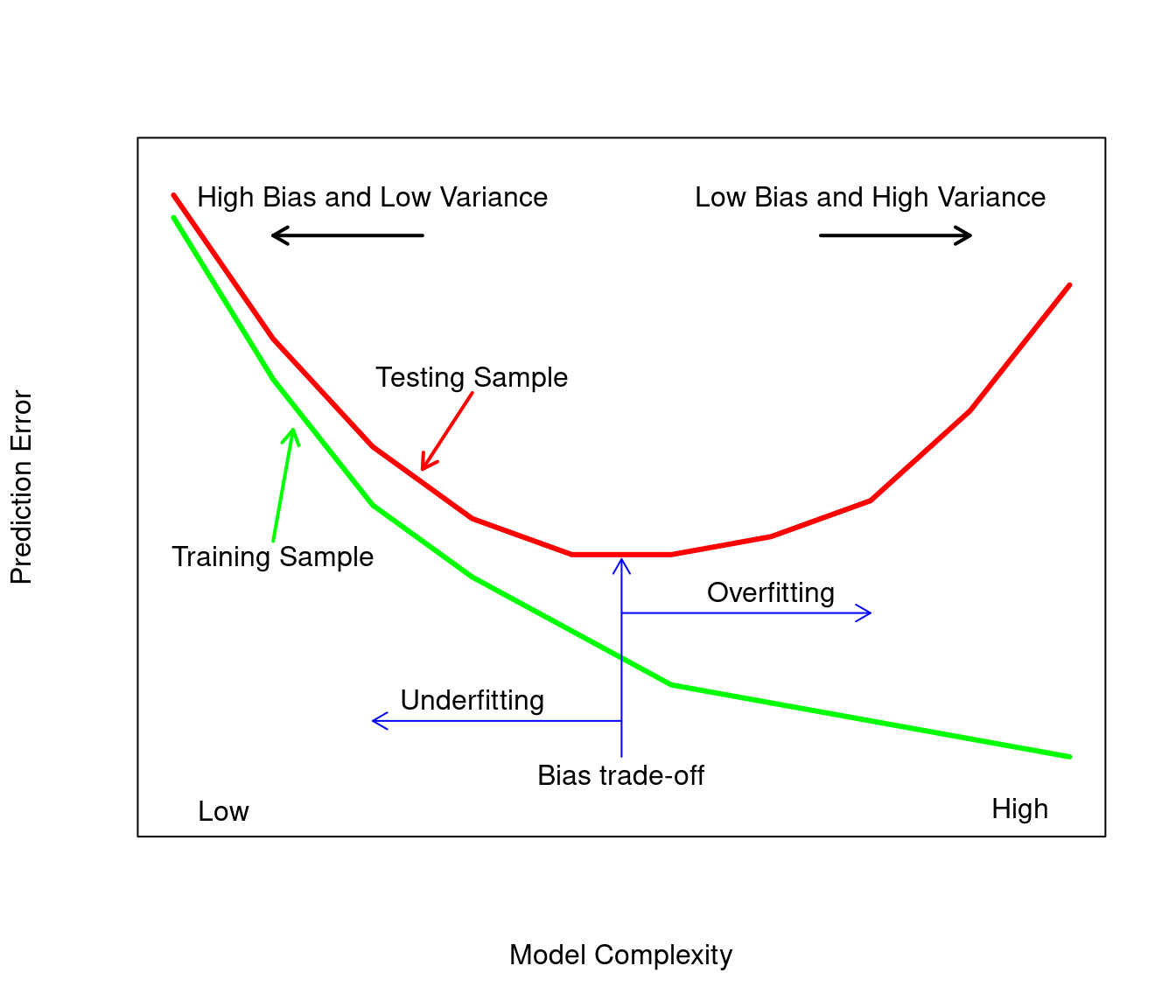
Figure 2.1: Modified schematic display of the bias variance based on Figure 2.11 of Hastie, Tibshirani, and Friedman (2009)