Chapter 4 Resampling Methods and Training Models

This Chapter will provide a brief introduction to resampling methods available in caret with a primary focus on cross validation. Models will subsequently be trained using the caret function train() using one of caret’s resampling methods to optimize the bias variance trade-off.

4.1 k-Fold Cross Validation

$k$-fold cross validation divides the data into $k$ subsets and performs the holdout method $k$ times. Specifically, one of the $k$ subsets is used as the test set and the other $k-1$ subsets are put together to form a training set. Figure 4.1 shows a schematic display of 5-fold cross-validation. The lightly shaded rectangles are the testing sets and the darker shaded rectangles are the training sets. The average MSE across all $k$ trials is computed and is denoted $\text{CV}_{(k)}$. Mathematically, the $k$-fold CV estimate is computed as shown in (4.1).

\[\begin{equation} \text{CV}_{(k)} = \frac{1}{k}\sum_{i = 1}^{k}\text{MSE}_i \tag{4.1} \end{equation}\]

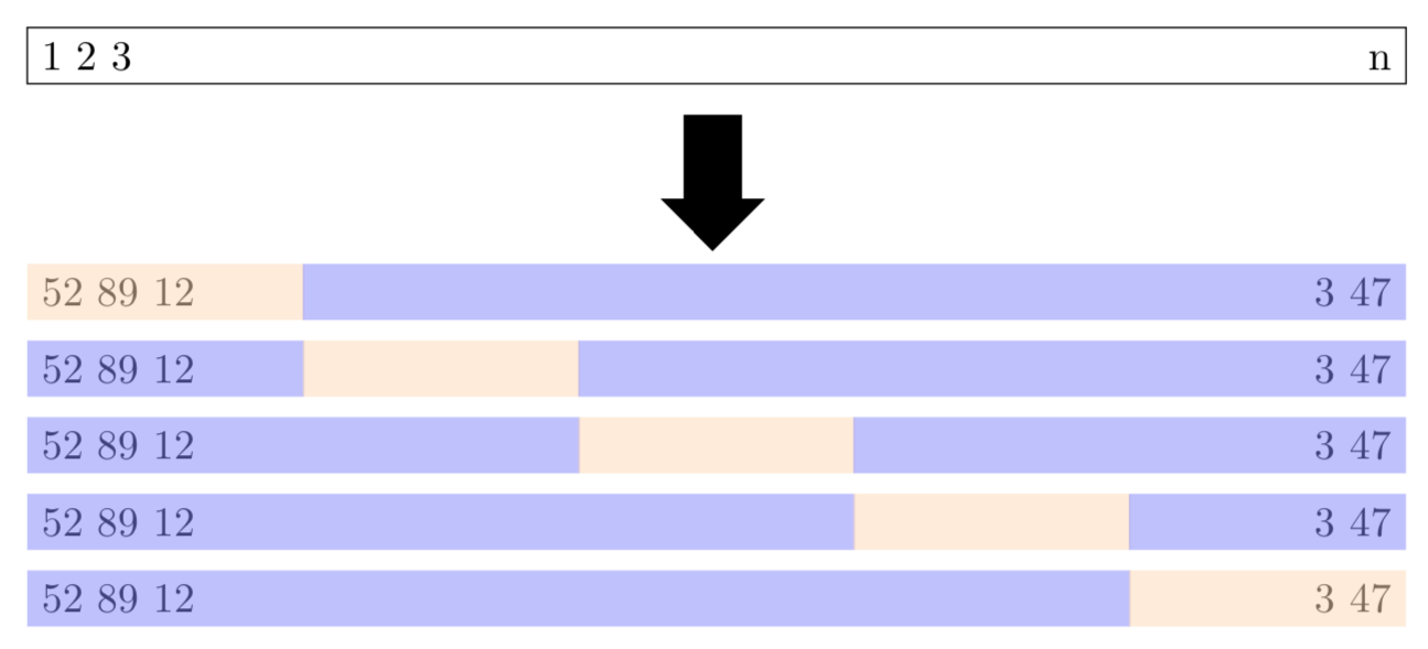
Schematic display of $5$-fold cross-validation based on Figure 5.5 in @james_introduction_2017. The lightly shaded rectangles represent the testing sets and the darker shaded rectangles represent the training data sets.

Figure 4.1: Schematic display of $5$-fold cross-validation based on Figure 5.5 in James et al. (2017). The lightly shaded rectangles represent the testing sets and the darker shaded rectangles represent the training data sets.

4.2 Resampling with caret

The trainControl() function from caret specifies the resampling procedure to be used inside the train() function. Resampling procedures include -fold cross-validation (once or repeated), leave-one-out cross-validation, and bootstrapping. The R code below creates a myControl object that will signal a 10-fold (number = 10) repeated five times (repeats = 5) cross-validation (method = "repeatedcv") scheme (50 resamples in total) to the train() function. The argument savePredictions = "final" saves the hold-out predictions for the optimal tuning parameters.

myControl <- trainControl(method = "repeatedcv",
                          number = 10,
                          repeats = 5,
                          savePredictions = "final")

4.3 Training Linear Models

To fit a model with a particular algorithm, the name of the algorithm is given to the method argument of the train() function. The train() function accepts a formula interface provided the data is also specified in the function. The R code below fits a linear model by regressing medv on all of the predictors in the training data set using the dot indicator which selects all predictors (medv ~ .). The preferred way to train a model is by passing the response vector to the y argument and a data frame of the predictors or a matrix of the predictors to the x argument of train(). Both approaches are shown below.

# Least Squares Regression
set.seed(31)
mod_lm <- train(medv ~ ., 
                data = trainingTrans,
                trControl = myControl,
                method = "lm")
set.seed(31)
mod_lm2 <- train(y = trainingTrans$medv,     # response
                 x = trainingTrans[, 1:13],  # predictors
                 trControl = myControl, 
                 method = "lm")
mod_lm2

Linear Regression 

407 samples
 13 predictor

No pre-processing
Resampling: Cross-Validated (10 fold, repeated 5 times) 
Summary of sample sizes: 366, 367, 367, 365, 367, 366, ... 
Resampling results:

  RMSE      Rsquared   MAE     
  4.513069  0.7653955  3.328636

Tuning parameter 'intercept' was held constant at a value of TRUE

The average root mean squared error (RMSE) of the 50 resamples is 4.5131. Next, models using forward selection and backwards elimination algorithms from the leaps package are built using the train() function. Note that models in the previous R code as well as those created below are parametric estimators that assume the functional form of $f$ is linear.

# Forward Selection
set.seed(31)
mod_FS <- train(y = trainingTrans$medv,     # response
                x = trainingTrans[, 1:13],  # predictors
                trControl = myControl,
                method = "leapForward")
# Rearrange output and round answers to 4 decimals
round(mod_FS$results[, c(1, 2, 5, 3, 6, 4, 7)], 4)

  nvmax   RMSE RMSESD Rsquared RsquaredSD    MAE  MAESD
1     2 5.4768 0.8985   0.6580     0.0989 4.0332 0.5210
2     3 5.1777 0.9310   0.6931     0.1019 3.7640 0.4850
3     4 4.8272 0.8438   0.7335     0.0874 3.5446 0.4698

# Number of variables for min RMSE
mod_FS$bestTune

  nvmax
3     4

The R code above uses forward selection to create a model with 4 variables and returns an average RMSE of 4.8272.

# Backward Elimination
set.seed(31)
mod_BE <- train(y = trainingTrans$medv,     # response
                x = trainingTrans[, 1:13],  # predictors
                trControl = myControl,
                method = "leapBackward")
# Rearrange output and round answers to 4 decimals
round(mod_BE$results[, c(1, 2, 5, 3, 6, 4, 7)], 4)

  nvmax   RMSE RMSESD Rsquared RsquaredSD    MAE  MAESD
1     2 5.4780 0.8973   0.6572     0.0979 4.0423 0.5345
2     3 5.2401 0.9397   0.6849     0.1048 3.8133 0.5231
3     4 4.8603 0.8658   0.7295     0.0915 3.5711 0.4918

# Number of variables for min RMSE
mod_BE$bestTune

  nvmax
3     4

The R code above uses backward elimination to create a model with 4 variables and returns an average RMSE of 4.8603. The R code below uses the default arguments for the train() function with 10-fold cross validation repeated 5 times to determine the best constrained linear regression model.

# Elastic net
set.seed(31)
mod_EN <- train(y = trainingTrans$medv,     # response
                x = trainingTrans[, 1:13],  # predictors
                trControl = myControl,
                method = "glmnet")
# Rearrange output and round answers to 4 decimals
round(mod_EN$results[, c(1, 2, 3, 6, 4, 7, 5, 8)], 4)

  alpha lambda   RMSE RMSESD Rsquared RsquaredSD    MAE  MAESD
1  0.10 0.0148 4.5106 0.8207   0.7656     0.0798 3.3181 0.4711
2  0.10 0.1485 4.5065 0.8447   0.7659     0.0826 3.2861 0.4625
3  0.10 1.4846 4.7300 0.9921   0.7498     0.1061 3.3108 0.4631
4  0.55 0.0148 4.5111 0.8198   0.7656     0.0797 3.3199 0.4714
5  0.55 0.1485 4.5283 0.8692   0.7642     0.0858 3.2900 0.4633
6  0.55 1.4846 5.1240 0.9871   0.7167     0.1112 3.6431 0.4806
7  1.00 0.0148 4.5107 0.8219   0.7656     0.0799 3.3175 0.4711
8  1.00 0.1485 4.5707 0.9013   0.7602     0.0902 3.3063 0.4712
9  1.00 1.4846 5.3162 0.9452   0.7088     0.1024 3.7889 0.5095

# Tuning parameters for min RMSE
mod_EN$bestTune

  alpha    lambda
2   0.1 0.1484627

The best constrained regression model from the R code above has an average RMSE value of 4.5065 for $\alpha = 0.1$ and $\lambda = 0.1485$. To compare the four models (mod_LM, mod_FS, mod_BE, mod_EN) using the default performance metrics (MAE, RMSE, and $R^2$) one can pass a list of the trained models to the caret function resamples() as shown in the R code below or create the side-by-side boxplots shown in Figure 4.2.

ANS <- resamples(list(LM = mod_lm, BE = mod_BE, 
                      FS = mod_FS, EN = mod_EN))
summary(ANS)


Call:
summary.resamples(object = ANS)

Models: LM, BE, FS, EN 
Number of resamples: 50 

MAE 
       Min.  1st Qu.   Median     Mean  3rd Qu.     Max. NA's
LM 2.621662 2.977326 3.365617 3.328636 3.584517 4.733398    0
BE 2.791828 3.266337 3.486400 3.571124 3.758311 5.345722    0
FS 2.791828 3.247508 3.468883 3.544616 3.758311 4.944021    0
EN 2.620944 2.971925 3.285503 3.286104 3.498264 4.663030    0

RMSE 
       Min.  1st Qu.   Median     Mean  3rd Qu.     Max. NA's
LM 3.314638 3.917210 4.215800 4.513069 5.161295 6.289300    0
BE 3.761951 4.294390 4.630517 4.860255 5.352608 7.067993    0
FS 3.761951 4.236871 4.630517 4.827187 5.352608 6.646217    0
EN 3.319714 3.900138 4.227519 4.506550 5.197790 6.317780    0

Rsquared 
        Min.   1st Qu.    Median      Mean   3rd Qu.      Max. NA's
LM 0.5808695 0.7056142 0.7878469 0.7653955 0.8203268 0.8868594    0
BE 0.5117098 0.6854005 0.7592982 0.7295103 0.7903249 0.8684039    0
FS 0.5133736 0.6926438 0.7592982 0.7334605 0.7903249 0.8684039    0
EN 0.5707466 0.7050455 0.7934414 0.7659425 0.8244371 0.8881846    0

bwplot(ANS, layout = c(1, 3), scales = "free", as.table = TRUE)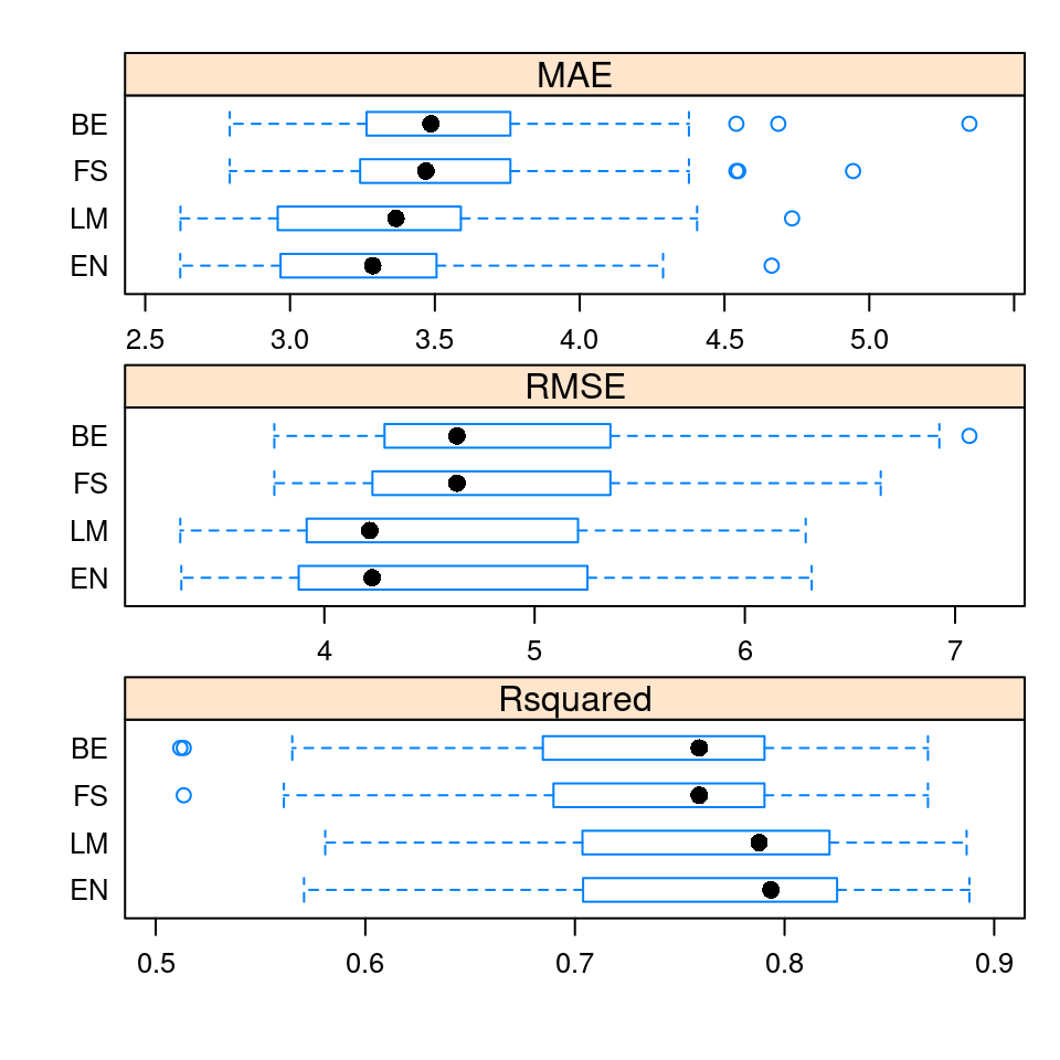

Figure 4.2: Boxplots of the default metrics for the 50 resamples in ANS

The default values for the Elasatic net code generated a grid with nine combinations of $\alpha$ and $\lambda$ values. To better tune the hyperparameters ($\alpha$, $\lambda$), the expand.grid() function is used to create a grid of $11 \times 8 =88$ combinations of alpha and lambda values that are assigned to the tuneGrid argument in the train() function of the R code below. The 88 different combinations of $\alpha$ and $\lambda$ are shown in Figure 4.3.

# Elastic net
set.seed(31)
mod_EN <- train(y = trainingTrans$medv,     # response
                x = trainingTrans[, 1:13],  # predictors
                trControl = myControl,
                method = "glmnet",
                tuneGrid = 
                  expand.grid(alpha = seq(0.1, 0.5, length = 11),
                              lambda = seq(0.08, 0.15, length = 8)))

print(plot(mod_EN, auto.key = list(title = "Regularization Parameter lambda", 
  space = "top", columns = 4), xlab = "Mixing Parameter alpha"))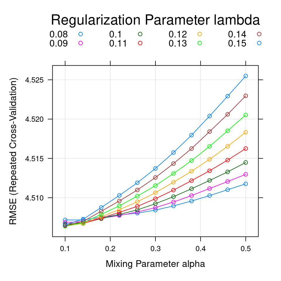

$The smallest RMSE (4.5064) was used to select the optimal model. The final values used for the model were $\alpha = 0.1$, and $\lambda = 0.13$.$

Figure 4.3: The smallest RMSE (4.5064) was used to select the optimal model. The final values used for the model were $\alpha = 0.1$, and $\lambda = 0.13$.

4.4 Training Nonlinear Models

To introduce regression trees, a tree is created to predict the response medv (median value of owner-occupied homes in $1000s) using only age as a predictor in the R code below. The stars after the output in R code below indicate a terminal node. Specifically, there are $n = 118$ homes greater than or equal to 92.3 years of age. The average medv for these 118 homes is 17.22 thousand dollars. There are $n = 195$ homes under 92.3 years of age but greater than 41.3 or more years of age. These 195 homes have an average medv of 23.36 thousand dollars. Finally, there are $n = 94$ homes under 41.3 years of age. The average medv for the $n = 94$ homes under 41.3 years of age is 27.72 thousand dollars. Figure 4.4 uses the partykit package to draw the regression tree. The code used to create Figure 4.4 is also shown below.

# Regression Tree
library(rpart)
set.seed(31)
mod_TRG <- rpart(medv ~ age, data = training)
mod_TRG

n= 407 

node), split, n, deviance, yval
      * denotes terminal node

1) root 407 35195.280 22.58968  
  2) age>=92.3 118  9411.559 17.22458 *
  3) age< 92.3 289 21000.340 24.78028  
    6) age>=41.3 195 13941.470 23.36359 *
    7) age< 41.3 94  5855.626 27.71915 *

library(partykit)
plot(as.party(mod_TRG))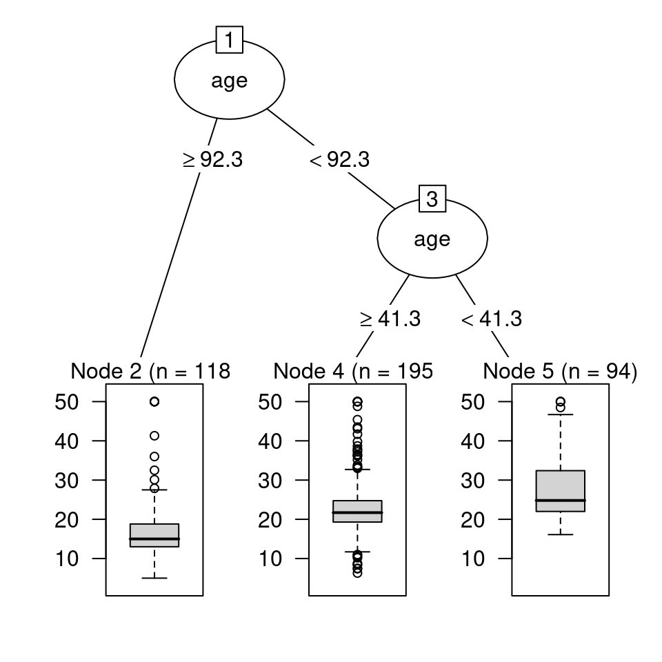

Figure 4.4: Regression tree for predicting medv based on age using the partykit package

A similar representation of the regression tree shown in Figure 4.4 is created with the rpart.plot package in the R code below and displayed in Figure 4.5.

rpart.plot::rpart.plot(mod_TRG)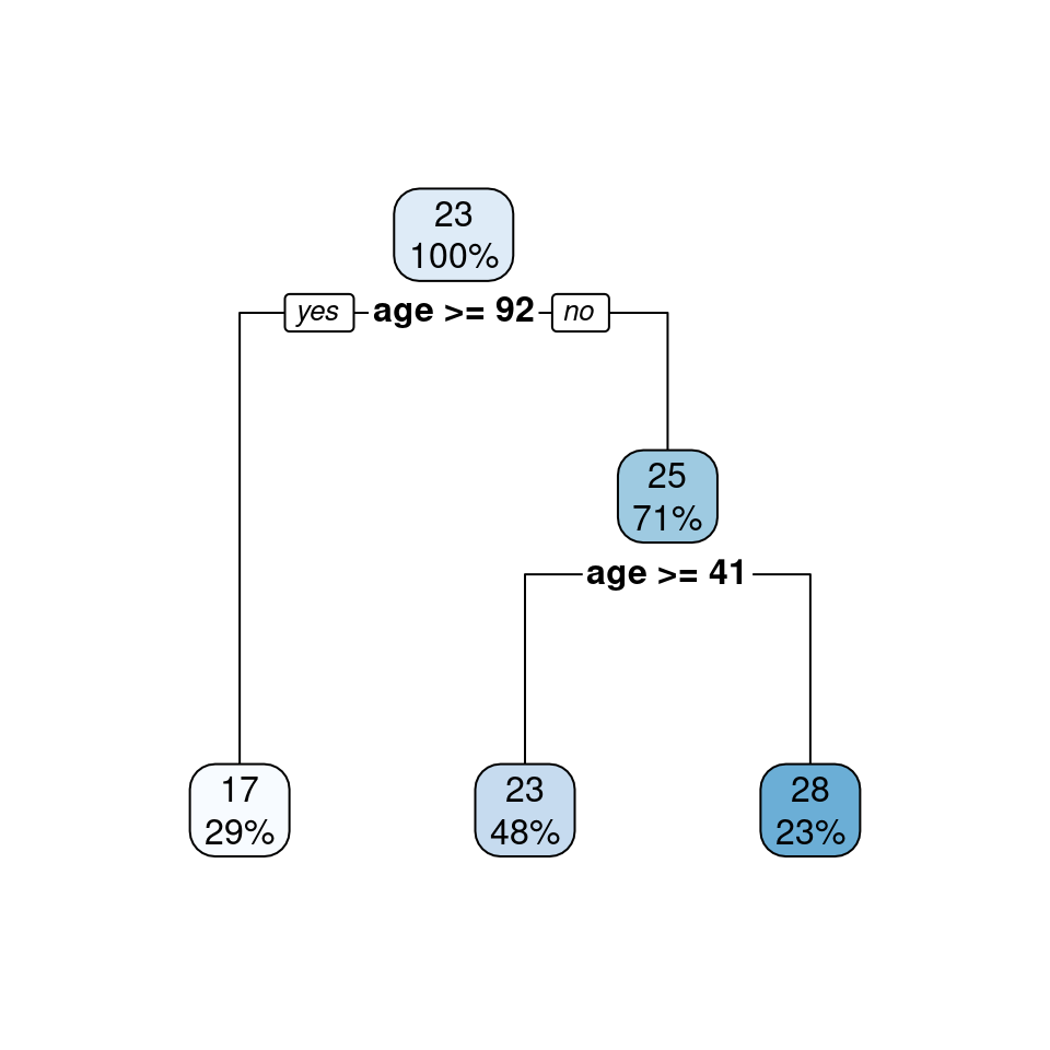

Figure 4.5: Regression tree for predicting medv based on age using the rpart.plot package

Figure 4.4 shows the distribution of the medv values with a boxplot in nodes 2, 4, and 5, while Figure 4.5 provides two numbers in each node: the mean of the medv values and the percent of the medv values in the node. For example, Figure 4.5 shows 29% of the values are in terminal node 2 and have an average of 17 thousand dollars; 48% of the values are in terminal node 4 and have an average of 23 thousand dollars; 23% of the values are in terminal node 5 and have an average of 28 thousand dollars.

The R code below uses the train() function from caret to determine the complexity parameter (cp) that results in the smallest RMSE when using all of the variables in trainingTrans. As the complexity parameter increases from zero, branches are pruned from the tree, reducing the complexity of the model in a fashion similar to how $\lambda$ controls the complexity of a linear model for the LASSO model given in (2.5).

# Regression Tree
set.seed(31)
mod_TR <- train(y = trainingTrans$medv, 
                x = trainingTrans[, 1:13],
                trControl = myControl,
                method = "rpart",
                tuneLength = 10)
# Rearrange output and round answers to 4 decimals
round(mod_TR$results[, c(1, 2, 5, 3, 6, 4, 7)], 4)

       cp   RMSE RMSESD Rsquared RsquaredSD    MAE  MAESD
1  0.0085 4.6512 1.1386   0.7466     0.1222 3.2081 0.5174
2  0.0104 4.7394 1.1410   0.7382     0.1261 3.2710 0.5354
3  0.0133 4.8107 1.1337   0.7307     0.1276 3.3591 0.5283
4  0.0185 4.8991 1.1807   0.7186     0.1337 3.4380 0.5221
5  0.0249 5.0710 1.1704   0.6983     0.1356 3.6035 0.5708
6  0.0259 5.0821 1.1787   0.6965     0.1358 3.6225 0.5722
7  0.0326 5.1043 1.2220   0.6906     0.1460 3.6786 0.5861
8  0.0673 5.6529 1.0976   0.6310     0.1437 4.0645 0.5826
9  0.1640 6.4335 1.2757   0.5225     0.1950 4.7216 0.8063
10 0.4800 8.5716 1.3843   0.3140     0.1093 6.2366 0.9024

# Complexity parameter for min RMSE
mod_TR$bestTune

           cp
1 0.008491945

Once the optimal complexity parameter is determined from cross-validation, a regression tree is grown using all of the transformed predictors in trainingTrans in the R code below and subsequently graphed in Figure 4.6 . If the user wants to create a random forest, which is a collection of decorrelated trees, the method argument in the train() function would be one of either rf or ranger.

# Regression Tree
library(rpart)
mod_TR3 <- rpart(trainingTrans$medv ~ ., 
                 data = trainingTrans, cp = mod_TR$bestTune)
rpart.plot::rpart.plot(mod_TR3)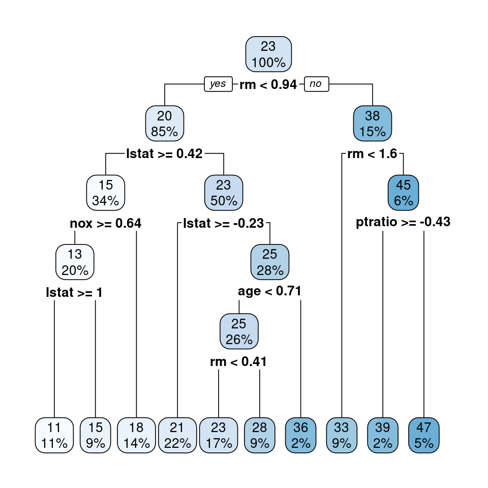

Figure 4.6: Regression tree for predicting medv based on all predictors in trainingTrans

The R code below creates a support vector regression model using a radial basis kernel.

set.seed(31)
mod_SVR <- train(y = trainingTrans$medv, 
                 x = trainingTrans[, 1:13],
                 trControl = myControl,
                 method = "svmRadial")
mod_SVR$bestTune

       sigma C
3 0.08108703 1

# Rearrange output and round answers to 4 decimals
round(mod_SVR$results[, c(1, 2, 3, 6, 4, 7, 5, 8)], 4)

   sigma    C   RMSE RMSESD Rsquared RsquaredSD    MAE  MAESD
1 0.0811 0.25 4.5649 1.1721   0.7833     0.1032 2.7560 0.4361
2 0.0811 0.50 4.1217 1.1543   0.8137     0.1001 2.5069 0.4032
3 0.0811 1.00 3.7160 1.1150   0.8408     0.0952 2.3499 0.3710

Using the default arguments for svmRadial indicates a cost (C) of 1 and a sigma of 0.0811 yields an average RMSE value of 3.716. A grid of 77 combinations of C and sigma is used to tune the hyperparameters of the support vector regression model in the R code below.

set.seed(31)
mod_SVR <- train(y = trainingTrans$medv, 
                 x = trainingTrans[, 1:13],
                 trControl = myControl,
                 method = "svmRadial",
                 tuneGrid = expand.grid(C = seq(1, 21, length = 11), 
                            sigma = seq(0.021, 0.081, length = 7)))
mod_SVR$bestTune

   sigma  C
45 0.041 13

min(mod_SVR$results$RMSE)

[1] 3.149087

By tuning the hyperparameters of the support vector regression model in the R code above, the support vector regression model achieves an average RMSE of 3.1491.

The R code below creates a random forest using the default arguments for method = "rf".

set.seed(31)
mod_RF <- train(y = trainingTrans$medv, 
                x = trainingTrans[, 1:13],
                trControl = myControl,
                method = "rf")
mod_RF

Random Forest 

407 samples
 13 predictor

No pre-processing
Resampling: Cross-Validated (10 fold, repeated 5 times) 
Summary of sample sizes: 366, 367, 367, 365, 367, 366, ... 
Resampling results across tuning parameters:

  mtry  RMSE      Rsquared   MAE     
   2    3.671831  0.8546174  2.471371
   7    3.283247  0.8729520  2.246165
  13    3.386089  0.8627773  2.303298

RMSE was used to select the optimal model using the smallest value.
The final value used for the model was mtry = 7.

mod_RF$bestTune

  mtry
2    7

min(mod_RF$results$RMSE)

[1] 3.283247

Using the default arguments for rf returns an average RMSE value of 3.2832 when the parameter mtry = 7. The R code below attempts to improve the average RMSE value by tuning the parameter mtry.

set.seed(31)
mod_RF <- train(y = trainingTrans$medv, 
                x = trainingTrans[, 1:13],
                trControl = myControl,
                method = "rf",
                tuneGrid = expand.grid(mtry = seq(2, 9, 1)))
mod_RF$bestTune

  mtry
6    7

min(mod_RF$results$RMSE)

[1] 3.287956

By tuning mtry in the R code above, the random forest model achieves an average RMSE of 3.288.

The R code below creates a $k$-nearest neighbors model using the default arguments for method = "knn".

set.seed(31)
mod_KNN <- train(y = trainingTrans$medv, 
                 x = trainingTrans[, 1:13],
                 trControl = myControl,
                 method = "knn")
# Rearrange output and round answers to 4 decimals
round(mod_KNN$results[, c(1, 2, 5, 3, 6, 4, 7)], 4)

  k   RMSE RMSESD Rsquared RsquaredSD    MAE  MAESD
1 5 4.4191 1.0451   0.7889     0.1036 2.8824 0.3870
2 7 4.6052 1.0389   0.7741     0.1089 3.0331 0.4037
3 9 4.7805 1.0809   0.7571     0.1164 3.1342 0.4250

mod_KNN$bestTune

  k
1 5

Using the default arguments for knn returns an average RMSE value of 4.4191 when the parameter k = 5. The R code below attempts to improve the average RMSE value by tuning the parameter k.

set.seed(31)
mod_KNN <- train(y = trainingTrans$medv, 
                 x = trainingTrans[, 1:13],
                 trControl = myControl,
                 method = "knn",
                 tuneGrid = expand.grid(k = seq(2, 12, 1)))
# Rearrange output and round answers to 4 decimals
round(mod_KNN$results[, c(1, 2, 5, 3, 6, 4, 7)], 4)

    k   RMSE RMSESD Rsquared RsquaredSD    MAE  MAESD
1   2 4.1019 0.9504   0.8068     0.0917 2.6999 0.3984
2   3 4.3240 1.0869   0.7893     0.1017 2.7685 0.4645
3   4 4.4326 1.1041   0.7818     0.1061 2.8598 0.4318
4   5 4.4191 1.0451   0.7889     0.1036 2.8824 0.3870
5   6 4.5004 1.0584   0.7816     0.1092 2.9638 0.3989
6   7 4.6052 1.0389   0.7741     0.1089 3.0331 0.4037
7   8 4.6817 1.0718   0.7662     0.1160 3.0879 0.4137
8   9 4.7805 1.0809   0.7571     0.1164 3.1342 0.4250
9  10 4.8270 1.1160   0.7520     0.1196 3.1596 0.4456
10 11 4.8511 1.1141   0.7518     0.1205 3.1756 0.4522
11 12 4.8931 1.1278   0.7480     0.1221 3.1981 0.4682

mod_KNN$bestTune

  k
1 2

By tuning k in the R code above, the $k$-nearest neighbors model achieves an average RMSE of 4.1019. The resamples() function is used in the R code below to show the average RMSE for the eight models (four parametric and four nonparametric). To obtain the MAE or $R^2$ values, replace the line round(summary(ANS)[[3]]$RMSE,4) in the R code below with round(summary(ANS)[[3]]$MAE,4) or round(summary(ANS)[[3]]$Rsquared,4) to obtain the MAE or $R^2$ values, respectively. Using the modelCor() function on the object ANS computes the correlation between each of the eight models.

ANS <- resamples(list(LM = mod_lm, BE = mod_BE, 
                      FS = mod_FS, EN = mod_EN,
                      TREE = mod_TR, SVR = mod_SVR,
                      RF = mod_RF, KNN = mod_KNN))
round(summary(ANS)[[3]]$RMSE, 4)

       Min. 1st Qu. Median   Mean 3rd Qu.   Max. NA's
LM   3.3146  3.9172 4.2158 4.5131  5.1613 6.2893    0
BE   3.7620  4.2944 4.6305 4.8603  5.3526 7.0680    0
FS   3.7620  4.2369 4.6305 4.8272  5.3526 6.6462    0
EN   3.3185  3.9003 4.2258 4.5064  5.1928 6.3142    0
TREE 3.0117  3.8021 4.4548 4.6512  5.4011 7.7048    0
SVR  1.9519  2.5009 2.7978 3.1491  3.6551 5.6453    0
RF   1.8148  2.6290 3.0499 3.2880  3.8251 6.3420    0
KNN  2.5415  3.4621 3.8008 4.1019  4.4898 6.8663    0

round(modelCor(ANS), 4)

         LM     BE     FS     EN   TREE    SVR     RF    KNN
LM   1.0000 0.8162 0.8225 0.9959 0.5060 0.5373 0.5857 0.3534
BE   0.8162 1.0000 0.9793 0.8430 0.5547 0.5525 0.5985 0.2954
FS   0.8225 0.9793 1.0000 0.8474 0.5356 0.5203 0.5936 0.3079
EN   0.9959 0.8430 0.8474 1.0000 0.5223 0.5550 0.6108 0.3560
TREE 0.5060 0.5547 0.5356 0.5223 1.0000 0.6768 0.7892 0.4910
SVR  0.5373 0.5525 0.5203 0.5550 0.6768 1.0000 0.7034 0.5141
RF   0.5857 0.5985 0.5936 0.6108 0.7892 0.7034 1.0000 0.4327
KNN  0.3534 0.2954 0.3079 0.3560 0.4910 0.5141 0.4327 1.0000

The dotplot() function creates plots of the mean estimated accuracy for all eight algorithms as well as individual 95% confidence intervals on the metrics for each algorithm as shown in Figure 4.7 which is created from the R code below.

dotplot(ANS, scales = "free", layout = c(1, 3))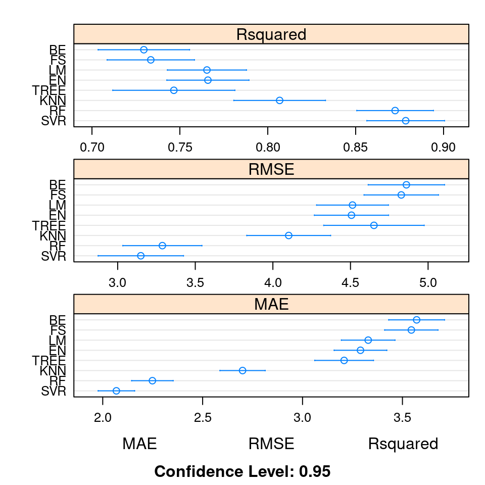

Figure 4.7: Comparison of $R^2$, RMSE, and MAE for eight different algorithms used to predict medv from the Boston data set

References

James, Gareth, Daniela Witten, Trevor Hastie, and Robert Tibshirani. 2017. An Introduction to Statistical Learning: With Applications in R. 1st ed. 2013, Corr. 7th printing 2017 edition. New York: Springer.